Coordinates systems

A few definitions

Voxel: a 3D pixel in a bitmap image: in other words, a small cube, generally associated with a value. The value may have any type (float, int, RGB color, vector…). Generalizing the 3D concept, we may manupulate data in 4D, or more dimensions: the voxel there has more than 3 dimensions. A voxel has a size (dimension in mm), in each dimension. Voxels are assumed to be aligned in a grid in regular data we manipulate in neuroimaging.

Voxel size: floating point dimension of the voxel, in each dimension, in millimeters. May be 3D, 4D, or more. Only meaningful for “voxelized data”, bitmap images or “buckets”. A mesh has float coordinates, and thus does not have voxels nor a voxel size.

Coordinates: 3D position: 3 floating point numbers.

• Float coordinates: generally in millimeters.

• Voxel coordinates: In images or “buckets”, it may be given as int coordinates, that is voxel indices in a voxels grid (array, image, bucket). To get the “real world” float mm coordinates, voxel int coords normally just need to be multiplied with the voxel sizes. This assumes the real world origin is in the center of the “first” voxel in the array. The array orientation however, may differ between different conventions and arrangements, thus additional coordinates transformations may be required. (see later)

To be usable, coordinates must be associated with a coordinates system (a referential) which specifies where the origin is, and where the axes go.

Referential: a coordinates system. Generally only defined by an identifier (a name, or an UUID). A referential is relative to other referentials, thus is mainly defined by transformations to/from other referentials. However it may specify additional information, like where is the origin, where the axes go, how they are oriented, if it is “direct” or “indirect”.

• Direct referential: follows the “right hand rule”

• Indirect referential: opposite: one axis is contradicting the “right hand rule”.

For brain images, we often characterize axes orientations relatively to the head: AP (anterior to posterior) or PA, LR (left to right) or RL, SI (superior to inferior) or IS. To summarize the 3 axes we sometimes use the 3 initials of the directions axes are pointing to: RAS (X: to Right, Y: to Anterior, Z: to Superior), LAS, LPI, etc.

http://www.grahamwideman.com/gw/brain/orientation/orientterms.htm

Transformation: a mathematical operation allowing to transform coordinates from one referential to another referential. We normally use them in real world float mm coordinates, but going from voxels to mm may be represented as a transformation per se.

Coordinates systems

Mesh coordinates

Mesh coordinates are “simpler” because they are always real world mm coordinates. However their referential has to be specified.

When a mesh is built from meshing an object in a voxels volume (like a brain segmentation) using the AIMS Mesher (like the AimsMesh, AimsMeshBrain, AimsMeshWhite commands), then the mesh referential is the AIMS referential of the volume data, in mm (see below).

Meshes obtained by other software, like Freesurfer, may reside in different referentials.

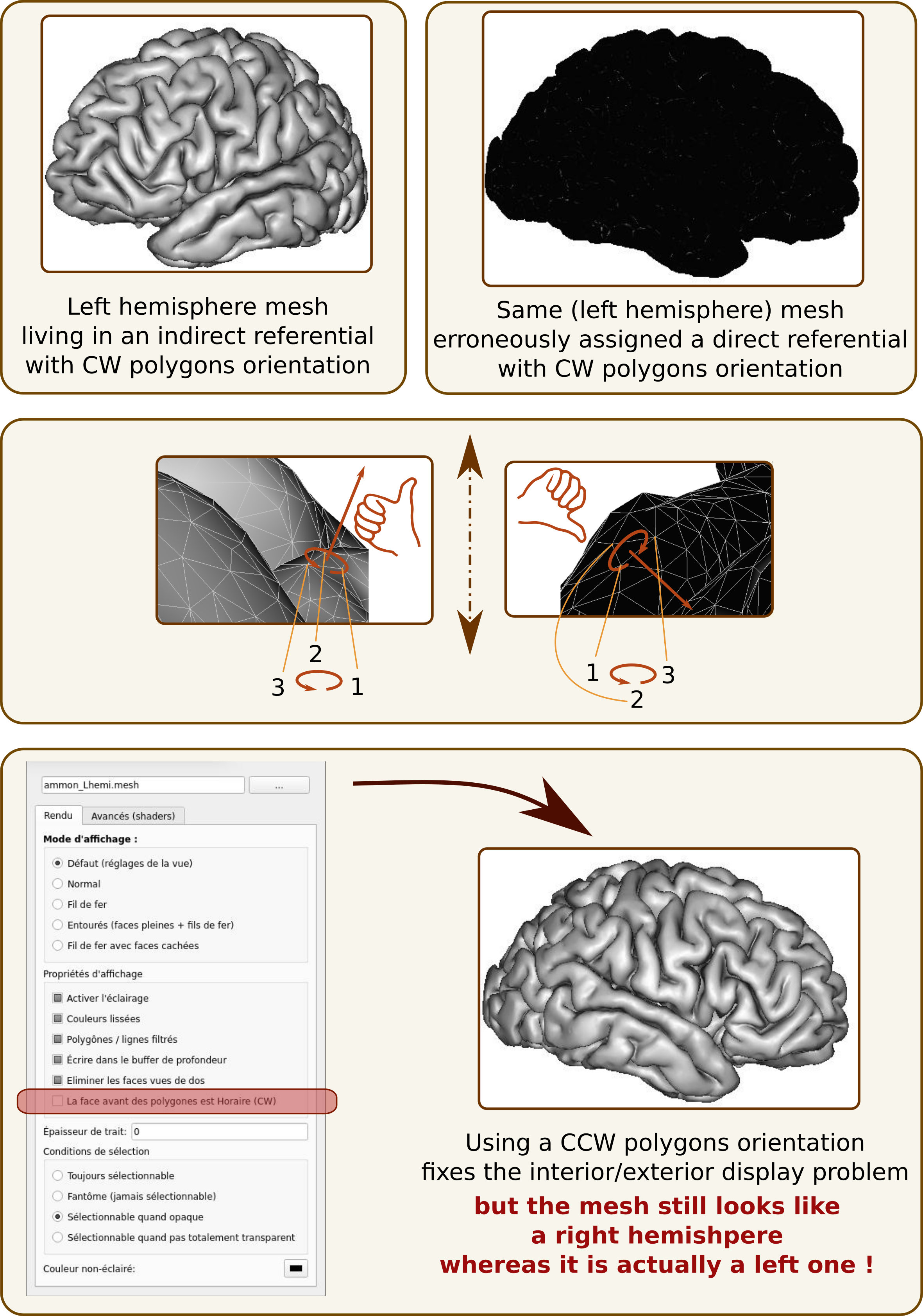
Direct and indirect referentials for meshes

A mesh is composed of, at least, vertices (points with 3D positions) and polygons (list of vertices forming a face - generally triangles, that is 3 vertices per polygon). The orientation of vertices in a polygon indicates which side of the polygon is the “exterior” of the mesh. Rendering software may display differently internal and external sides of meshes, or not render at all the internal side for optimization purposes. This is the default in several software, including Anatomist.

The external side of a polygon is determined by a “counter-clockwise” or “clockwise” parameter, and the right hand rule (see here, the section “Curve orientation and normal vectors”).

Meshes may provide normal vectors, which are supposed to point to the outside direction.

If a mesh resides in a direct referential, but is interpreted as being coordinates in an indirect referential (or the contrary), then the inside and outside notions will be reversed, and meshes will not be rendered correctly:

• polygons will likely appear black or invisible

• the mesh will appear as symmetrical to what it is: typically a left hemisphere mesh will look like a right one, and the contrary, which can lead to dramatic mistakes.

Volume coordinates

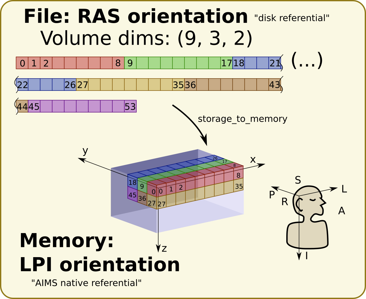
The volume case is much more complex: volumes use voxels. Voxels are data arrays, and the order voxels are stored can matter. Different software may interpret their order differently. Different file formats may store them differently.

For instance, NIFTI files allow to store voxels data in any order (x rows as contiguous data on disk, then y columns, then z slices, with RAS orientation or any other). Their orientation is actually known only in the transformations between this “disk voxels order” to known referentials (like MNI ICBM, or a “scanner” referential with known axes orientation). If no transformation is specified in the file, then voxels order is unknown, which is wrong.

The “Scanner-based coordinates” referential in NIFTI files is always assumed to be in RAS orientation, like the MNI ICBM one.

Some software use natively the “disk voxels orientation”, like SPM or Nibabel. Some other use a constant orientation in computer memory, like AIMS and Anatomist. Thus there is a transformation between the disk orientation and the memory orientation (this transformation, contrarily to most others, is working in voxel int coordinates).

AIMS is always loading data in memory in a constant orientation, namely a “LPI” orientation.

Note that this referential is indirect.

An example:

Then there may exist transformations between the memory referential and other referentials.

Note that a volume is an array of voxels with given dimensions: int voxels coordinates must fit into a bounding box, with positive indices, and must not exceed the dimension of the volume array, otherwise data will end up outside of the volume storage, which will result in lost data (at best), or programs crashes…

AIMS conventions

AIMS always loads voxel data in a “LPI” orientation, as said above. This has pros and cons, but is consistent, format-independent, and allows to use simple operations like “imageA + imageB”.

Information in AIMS headers are normalized the following way in the following header properties:

• referential: the identifier of the AIMS (LPI) referential of the data in its native space.

• storage_to_memory: transformation matrix (rotation/flip only) from the disk storage voxels orientation space to the AIMS referntial of the data. Applied to int voxels coordinates, the matrix only contains -1, 0 and 1 values, plus a translation to compensate filpped axes.

• referentials: (note the s at the end) list of referential IDs (or names) toward which transformations are provided.

• transformations: list of affine transformation matrices. There should be the same number of transformations as there are items in the referentials list. Each transformation goes from the AIMS referential of the data to the referential item at the same position in the referentials list.

The AIMS referential is a convention for AIMS and only software based on AIMS, like Anatomist. Other software do not necessarily follow the same convention (and actually, no other software does). So transforms here cannot be simply passed to other software: they have to be converted (combined with other transformations) to go from/to other software conventions.

Data formats, as said above, use their own conventions and orientations to store voxels on disk. The transforms provided with AIMS headers always try to correctly convert transformations to get to/from the AIMS referential of the data.

To convert from/to software which are working in the disk storage orientation, the storage_to_memory matrix may be used.

Note that the AIMS internal convention is LPI orientation is an indirect referential, and is the “contrary” to the standard MNI ICBM referential, which is a direct referential. All 3 axes directions are flipped. But the axes orientations are the same (1st axis, “x” is left/right, “y” is anterior/posterior, “z” is superior/inferior). Thus transformation matrices contain negative numbers on their diagonal.

Specifying transformations in AIMS

A transformation may be found at different places:

• as part of a data file header: NIFTI (volumes) and GIFTI (meshes) formats can provide transformations from the data space to other coordinates systems. AIMS provides them following its conventions (see AIMS conventions above) in data objects header properties.

• an affine transormation file. AIMS uses the .trm format, which is a very simple text file specifying the matrix as 12 coefficients:

  Tx	Ty	Tz
  R11	R12	R13
  R21	R22	R23
  R31	R32	R33

  Tx, Ty, Tz are the translation coefficients, and R11.. R33 are the linear matrix cooefficients.

• a vector field for non-linear transformations (free form or “FFD” deformations) which are generally stored in 3D volumes containing a displacement vector (3 coordinates) in each voxel, or a 5D NIFTI volume file where the 5th dimension has size 3 and provides the displacement vectors coordinates.

• a combnination of such transformations, given “by hand”

• in a transformation graph (which may be a YAML or JSON file). See the dedicated section for transformation graph.

AIMS commands (like AimsApplyTransform) which take transformations as inputs, and the Reader API in C++ and Python languages can accept all these forms, with the following syntax. Note that some commands and functions allow only affine transformations. The syntax is illustrated as using the PyAims python API, but the same “filenames” can be given to the commands options.

See also: AIMS IO system.

• transformation filename with extension, either filename.trm for an affine transform, or filename.ima or filename.nii.gz for a vector field:

  from soma import aims, aimsalgo
  # aimsalgo is needed because FFD vector fields are defined there, and not
  # in aims(data)
  
  transform = aims.read('filename.trm')
  # or, to take the inverse:
  transform_inv = aims.read('filename.trm?inv=1')
  # for vector field we must provide dtype to avoid confusion with reading a
  # volume object, since it's the same file
  ffd_trans = aims.read('filename.ima', dtype='Transformation3d')
  

• transformation in a data file header, using the “fake extension” .trmhdr:

  # take the 1st transform in the header
  transform = aims.read('filename.nii.trmhdr')
  # or, to be more precise, or take the 2nd transform:
  transform2 = aims.read('filename.nii.trmhdr?index=1')
  # or, to take the inverse of the 2nd transform:
  transform2_inv = aims.read('filename.nii.trmhdr?index=1&inv=1')
  

• composition of transformations: they will be composed using the composition operator (̀`*`), using the “fake extension” .trmc:

  transform = aims.read('file1.trm?inv=1*file2.nii.trmhdr?index=1.trmc?')
  

  Note that, here, the tailing ? is needed to avoid a parsing error: if we don’t supply it, the IO system will parse the filename as file1.trm?inv=1*file2.nii.trmhdr with options {"index": "1.trmc"}, which is not what we want here.

• transformation between two identified referentials in a transormations graph (see Transformation graph below):

  transform = aims.read('graph.yaml?source=MNI Colin 27&dest=MNI 152 ICBM 2009c Nonlinear Asymmetric')
  

Transformation graph

Graph

Transformations graphs have been introduced in Aims 5.1 (in 2022). A transformation graph is a structure which stores referentials and transformations between them, and allow to simplify access to them. They perform automatic composition, and inversion when possible, and can provide a transformations path between two given referentials, either as a composed transformation, or a composition chain.

The graph describes the transformations graph structure, and performs lazy loading of transformation files, and composition when needed along a path. Composed (deduced) paths are stored in the graph in order to speed up later access.

Individual transformations may be in any of the formats specified in the above section Specifying transformations in AIMS.

The graph structure is a dictionary-like object, which can be read from a JSON or a YAML file, or even a MINF file - actually any file format which can be read as a generic Aims Object (or a python dictionary). The dictionary should be organized as a 2-level dictionary:

{
    source_ref_id: {
        dest_ref_id1: transformation1,
        dest_ref_id2: transformation2,
    },
    ...
}

Transformations (here transformation1 and transformation2) may be either:

• file names (.trm for affine transformations, or .ima for vector fields, for instance, or .trmhdr or .trmc, see above)

• affine matrix written in a line vector, ex:

  {
      "source_ref": {
          "dest_ref": [1, 0, 0, 0,
                       0, 1, 0, 0,
                       0, 0, 1, 0,
                       0, 0, 0, 1]
      }
  }
  

• a transformation more complete description as a dictionary, containing an affine matrix as above, and possibly a header:

  {
      "source_ref": {
          "dest_ref": {
              "affine": [1, 0, 0, 0,
                         0, 1, 0, 0,
                         0, 0, 1, 0,
                         0, 0, 0, 1],
              "header": {
                  "free_field": "free value"
              }
          }
      }
  }
  

See the C++ API, or the Python API.

It can be loaded using the usual API:

graph = aims.read('graph.yaml')

Graphs may be saved also, using the API:

aims.write(graph, 'graph.yaml')

By default the graph is saved in a file, and each transformation is also saved in a separate file in the same directory. So it’s better to write in a new directory. Transformations with an existing file name (read previously) and saved at the same place wil overwrite older ones.

It is possible to specify write options:

allow_read: bool (default: true)

transformations not already loaded will be loaded before saving, which mean they will actually be saved. Otherwise only those already loaded will be saved.

affine_only: bool (default: false)

save only affine transformations

release_loaded: bool (default: false)

if allow_read is true, transformations will be released (unloaded) after they are saved, in order to avoid using memory (useful for non-linear vector fields)

embed_affines: bool (default: false)

do not write affine transformations in separate .trm files, but embedded in the graph file, with their matrix inside.

Ex:

aims.write(graph, 'graph.yaml',
           options={'embed_affines': True, 'allow_read': True})

Transformation

To obtain a transformation in a graph, use the getTransformation method, preferably after having loaded affine and inverse transforms in case the graph is incomplete:

graph.registerInverseTransformations(True)
tr = graph.getTransformation(
    'MNI Colin 27',
    'MNI 152 ICBM 2009c Nonlinear Asymmetric')

A transformation can be directly loaded from a graph file:

tr = aims.read('graph.yaml?source=MNI Colin 27&dest=MNI 152 ICBM 2009c Nonlinear Asymmetric')

which is equivalent to the above operations.

Thus if you frequently work with the same referentials and data with the same transformations chains, it’s convenient to write a graph file and reuse it later.

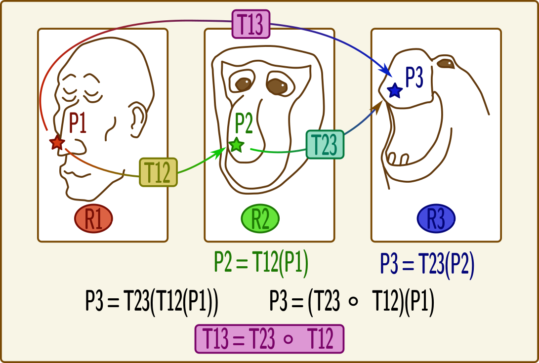
Combining transformations

Transformations can be combined, or composed to get coordinates from a “source” coordinates system to a “target” one, passing through intermediate referentials. To correctly transform coordinates, transformations should be combined “in reverse order”: transformations which should be applied first are on the “right” of the expression, and those which apply later are on the “left”.

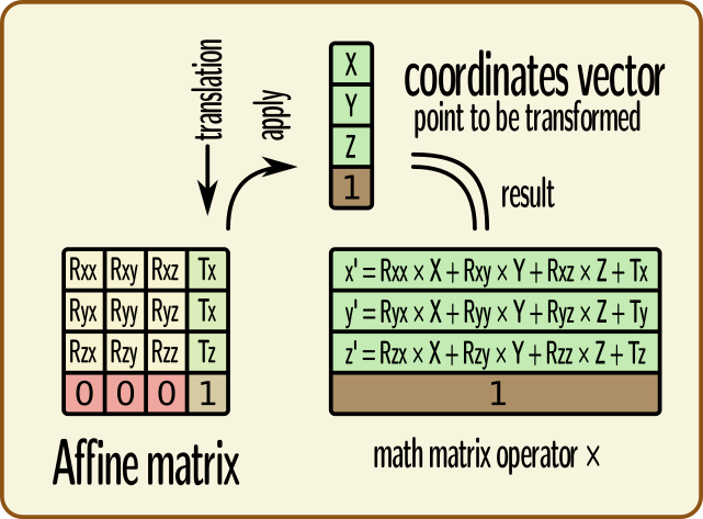
Affine transformations can be represented in matrix math shapes, as 4x4 matrices. Coordinates to be transformed are represented as colum vectors. The last line of an affine transformation matrix is normally (0, 0, 0, 1), the last column corresponds to the translation (origin shift) to be applied (the 4th coefficient of this column is 1, as it already appears on the last line). Coordinates vector are added a 4th component, which is 1.

For affine transformations, the composition operator is the mathematical matrix × operator (or * in C++ or Python languages), used in the same order. The result is also an affine transformation:

T12 = aims.read('transform_1_TO_2.trm')
T23 = aims.read('transform_2_TO_3.trm')
T13 = T23 * T12

For any type of 3D transformation, combining them is possible via the operator * in AIMS / PyAIMS. In C++, this API uses reference-counters:

#include <aims/io/reader.h>
#include <aims/transformation/transformation_chain.h>
#include <aims/transformation/affinetransformation3d.h>

using namespace carto;
using namespace soma;
using namespace aims;

int main()
{
  Reader<Transformation3d> r( "ffd.ima" ); // may be any type of transform
  rc_ptr<Transformation3d> t1( r.read() );

  affinetransformation3d *at2 = new affinetransformation3d;
  at2->affine()( 0, 0 ) = -1.;  // flip x axis
  at2->affine()( 0, 3 ) = 200.; // X translation
  rc_ptr<Transformation3d> t2( at2 );

  rc_ptr<Transformation3d> result = t1 * t2; // (t2 will apply first)
}

Or, in python:

from soma import aims, aimsalgo  # aimsalgo is needed to read non-lin trans

t1 = aims.read('ffd.ima')
t2 = aims.AffineTransformation3d()
t2.affine()[0, 0, 0, 0] = -1.
t2.affine()[0, 3, 0, 0] = 200.
result = t1 * t2

Note that in python especially, there is no difference between handling affine or non-affine transformations for the composition operator. Just the result has a different type (AffineTransformation3d if both operands are affine, or TransformationChain3d otherwise).

Resampling

When resampling an image (a volume), what is actually used is the inverse transformation, because we need to find out, for each voxel of the destination image, where it comes from in the source image. That’s why the command AimsApplyTransform takes the inverse transform (-I option) to perform volumes resampling.

Transforming a mesh, on the contrary, requires the direct transformation (each vertex is directly transformed).

Images normalized using SPM

SPM12 can perform normalization by either resampling the input volume to the template space, or by only writing (affine and non-linear) normalization information.

Volume resampled in target space

It should be already in the same space and field of view as the template image (most of the time the template is the MNI ICBM152). But:

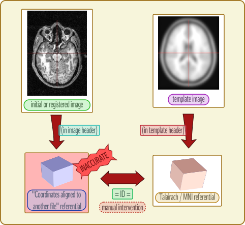
• SPM12 does not write the correct referential ID in the normalized NIFTI files. It used the code for “coordinates aligned to another file” (generic code in NIFTI format) instead of “MNI ICBM”. Thus the info is wrong, or at least inaccurate and unreliable, and we must get the transformation to this unspecified referential, and assume it’s actually MNI.

• It may be resampled with a different field of view, if specified. As we have seen, AIMS works in a referential which origin is “almost” in the corner of the image, thus two images differing on the field of view are not in the same space for AIMS. However both contain transformation information to a common space, namely the template MNI ICBM152. For normalized images, the transformation should be only a translation, plus the axes inversions for AIMS. To get from the resampled image to the template, the transform to be applied is thus the combination of both transformations (one inverted):

  template = aims.read('T1.nii')
  tr_index = template.header()['referentials'].index(
      aims.StandardReferentials.mniTemplateReferential())
  templ2icbm = template.header()['transformations'][tr_index]
  
  normalized = aims.read('wmri.nii')
  tr_index = -1  # assume the last transform is the one to ICBM (see above)
  norm2icbm = normalized.header()['transformations'][tr_index]
  
  norm2template = norm2icbm.inverse() * templ2icbm
  

SPM referentials representation

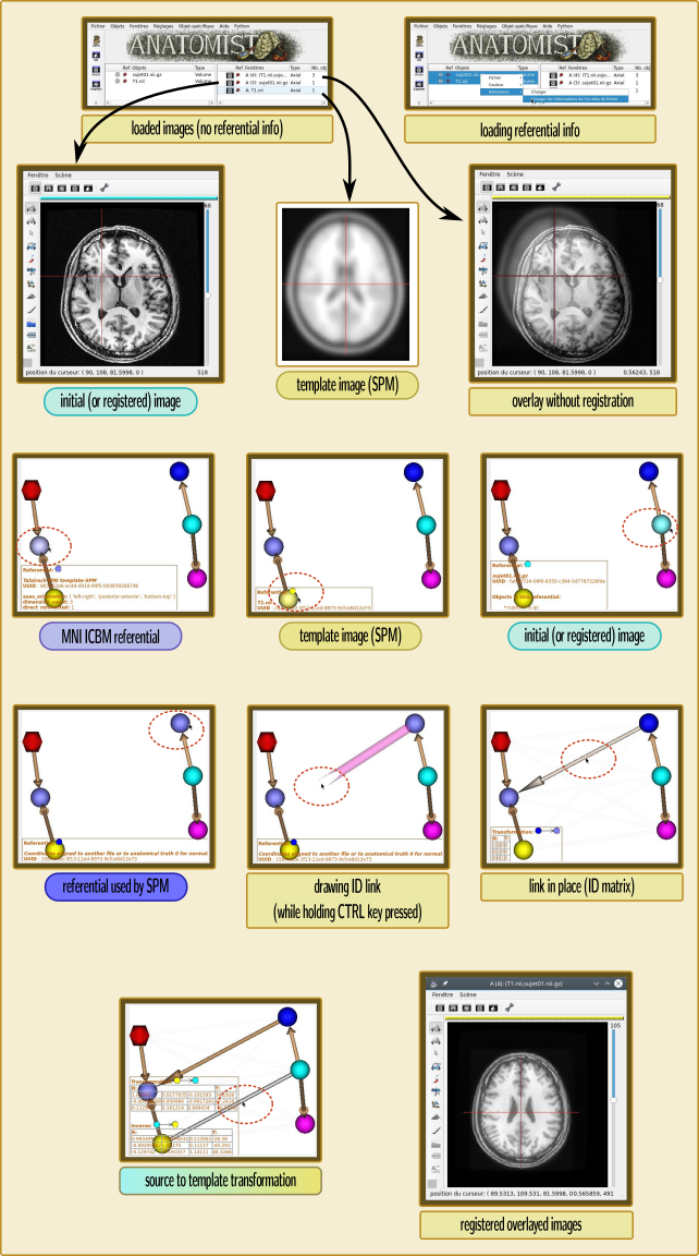
• For the same reason as the first point above (the referential ID is wrong in the normalized image), Anatomist will not apply the correct correspondance between images coordinates. It has to be specified manually, by telling him that the MNI ICBM referential and the “coordinates aligned to another file” for the normalized image are the same. This is done in the referentials window (menu “Settings / Referentials and transformations”), by “drawing” an arrow between these referentials, while holding the “Ctrl” key pressed (to tell that we want to add an “identity” transformation instead of loading a transformation file).

Manipulating Anatomist to get things in the correct referentials

At the end of the operation, if the input image is actually resampled to the template, the transformation between the initial and template volumes will just be a translation: the 3x3 linear submatrix will be Identity.

Normalization information not applied to an image

The affine part of the transformation is normally written back into the header of the source image by SPM (provided it is writable). Otherwise the transformation file is a matlab file with the suffix _sn.mat, and contains both an affine part (the same found in the source image), and a non-linear part.

Thus the source image is obviously not directly aligned to the template, but it has a transformation to the MNI space. So at the end, using it is exactly the same as the resampled volume case, except that the transformation in the source volume is not only a translation and axes inversions, but may include rotation, scaling etc.

The problems are exactly the same: the destination referential is wrong, and you have to know that the “coordinates aligned to another file” referential is the MNI ICBM, and thus you have to tell it to Anatomist to display them correctly.

At the end of the operation, the transformation between the initial and template volumes will not be only a translation, and may contain rotation, scaling, shearing, contrarily to the above resampled image use case.

FreeSurfer and AIMS coordinates systems

Use case: use Freesurfer meshes in Aims tools and the contrary.

Freesurfer uses (of course) different conventions and different coordinates systems from those used in AIMS…

Brainvisa proposes a “Freesurfer toolbox” which allows to read Freesurfer meshes and textures and to write them back in an “AIMS world” (in the Aims native coordinates system of the subject, like Morphologist meshes).

Freesurfer performs several resampling and coordinates systems changes during its main recon-all pipeline:

Freesurfer referentials and transformations

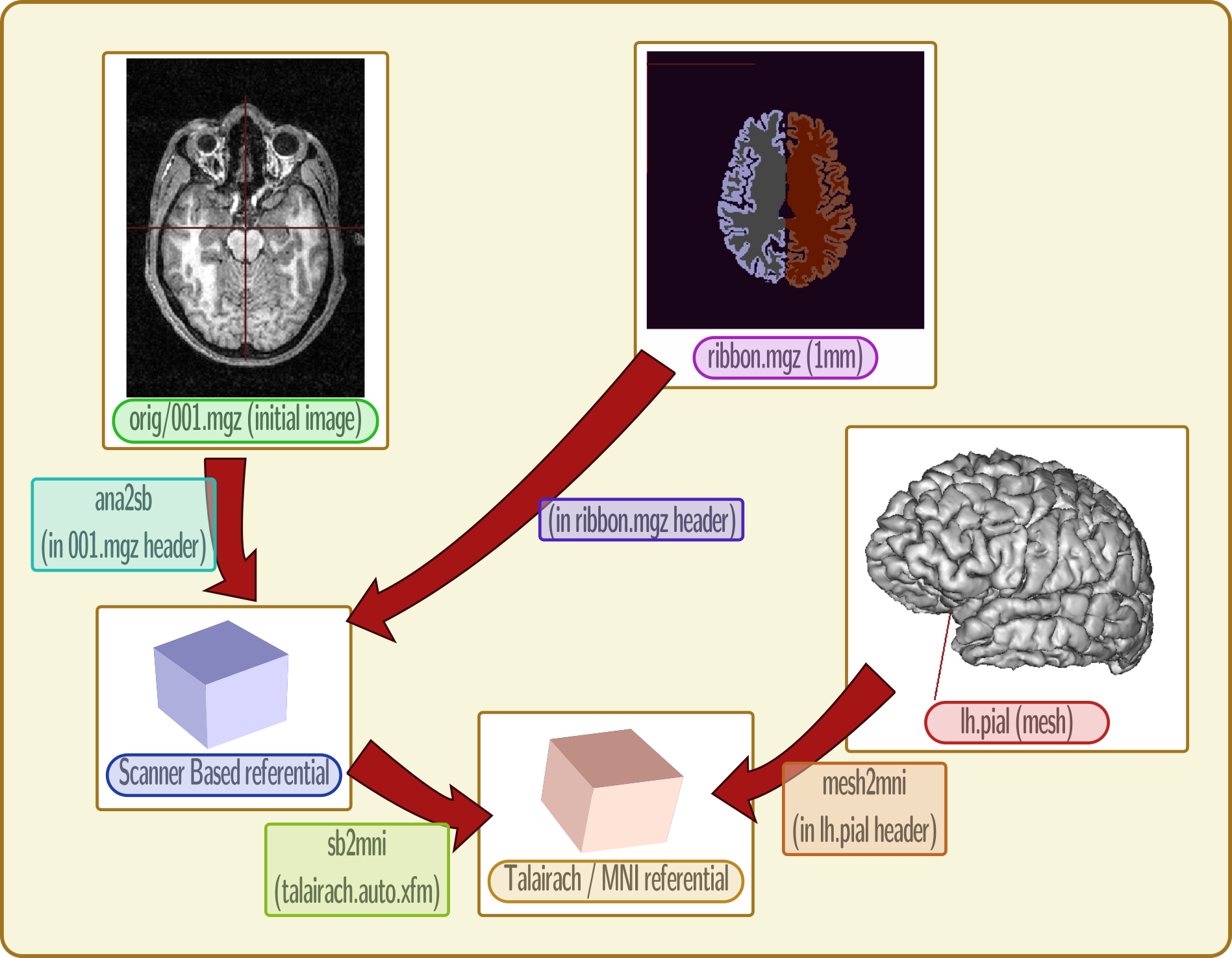
• raw image: orig/001.mgz

• transform to “scanner based referential” (direct, RAS oriented)

• resampling of T1 MRI to 1mm resolution: all processed images are in this shape: orig.mgz, ribbon.mgz etc.

• 1mm images also have a scanner-based referential and a transformation, which links to the orig/001.mgz image.

• normalization information to Talairach space: scanner-based to MNI space: transforms/talairach.auto.xfm

• meshes referential (direct, RAS)

• mesh to MNI transformation in meshes headers

• T1 MRI to meshes: Anat -> scanner (in MRI); Scanner -> MNI (from normalization); inverse(mesh -> MNI):

  anat2mesh = mesh2mni.inverse() * sb2mni * anat2sb