Anatomist user manual (2)

Combining objects

Objects superimposing

General definition

Objects superimposing consists in placing several objects in the same window. For example, you can superimpose hemispheres meshes or regions of interest with the matching anatomy (cf. examples below). So there is no specific menu to do that but you can change objects color to have a better display. For example, you can modify transparency, or lights on a mesh.

Be careful, superimposed objects must be in coherent referentials in order to get informative display. This means that if superimposed objects do not come from the same object (like hemispheres meshes that comes from a T1 MRI) or if they are non equivalent volumes (different subject, modality, point of view, voxels resolution…), you’ll probably have to load trnasformations between referentials in order to put all objects in the same coordinates system.

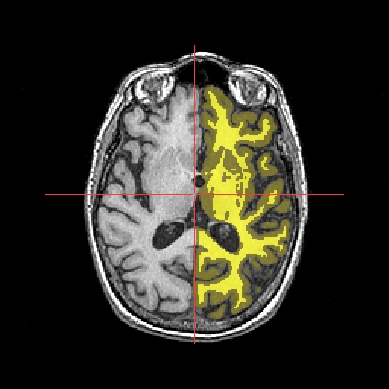
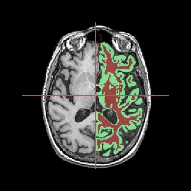
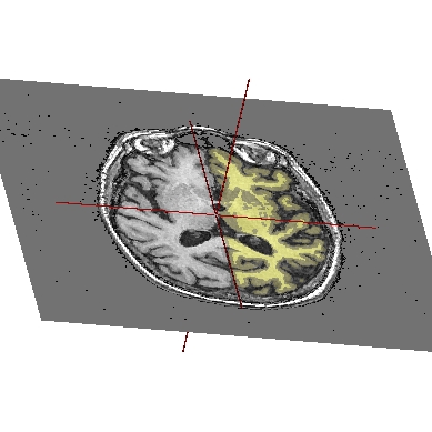
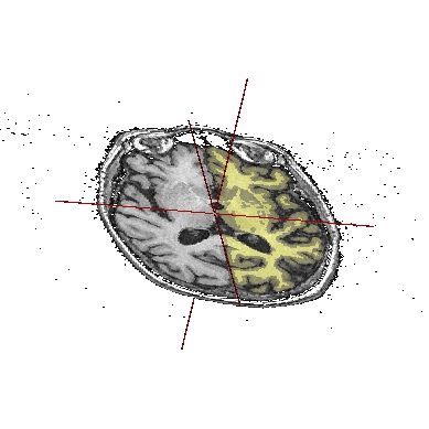
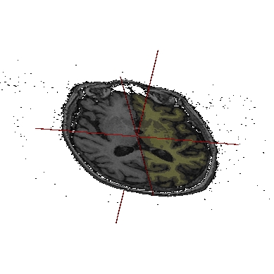
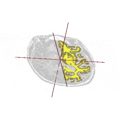
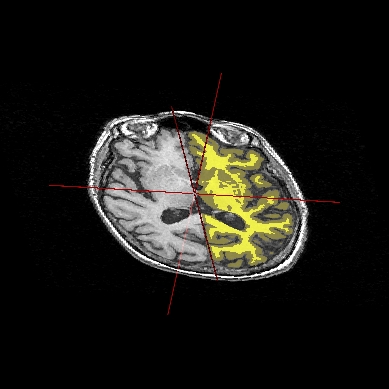
Application: Superimposing an anatomy and regions of interest (grey central nuclei)

In the following example, 3 objects are loaded in Anatomist:

• Object1 (O1): anatomy

• Object2 (O2): regions of interest graph drawn from the anatomy. So these 2 objects are in the same referential.

• Object3 (O3): nomenclature to associate colors to regions of interest according to their name. This object does not have to be put in a window. Link between names in the nomenclature and in regions of interest is done automatically by Anatomist.

These 2 objects are in the same coordinates system, so they will be placed in the same referential, that is to say they will have the same color circle (red by default).

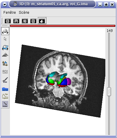
Superimposing an anatomy and regions of interest

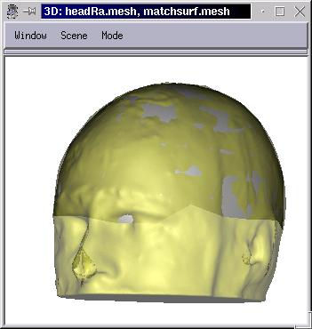
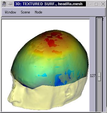
Application: Superimposing hemispheres meshes and head mesh

In the following example, 3 objects are loaded in Anatomist:

• Object1 (O1): head mesh, object obtained from a T1 MRI with BrainVISA anatomical pipeline. Opacity is decreased in the example below to enable visualization of the other objects.

• Object2 (O2): right hemisphere mesh, object obtained from the T1 MRI with BrainVISA anatomical pipeline.

• Object3 (O3): left hemisphere mesh, maillage de l’hemisphère gauche, object obtained from the T1 MRI with BrainVISA anatomical pipeline.

These three objects are in the same coordinates system, so they will be placed in the same referential, that is to say they will have the same color circle (red by default).

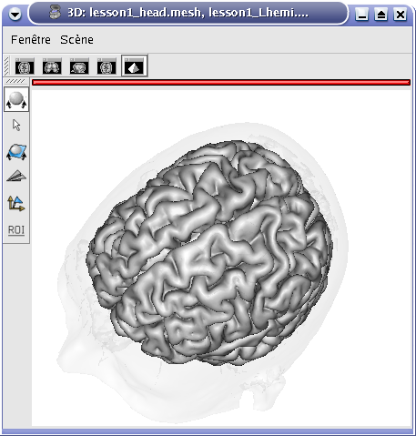
Superimposing hemispheres meshes and head mesh

Objects fusion

General definition

Objects fusion enables to create a new object from 2 or more other objects. Indeed, if you only put two volumes in the same window, you will see only one. To see the two volumes, you need to mix voxels from the two volumes in order to obtain a new volume. Note that fusionning more than 2 objects is only possible since 1.30 version. Besides, several new features have been added for fusion management. Several fusion combinations between objects are available,but for the moment, let’s see a fusion between two 3D volumes for example:

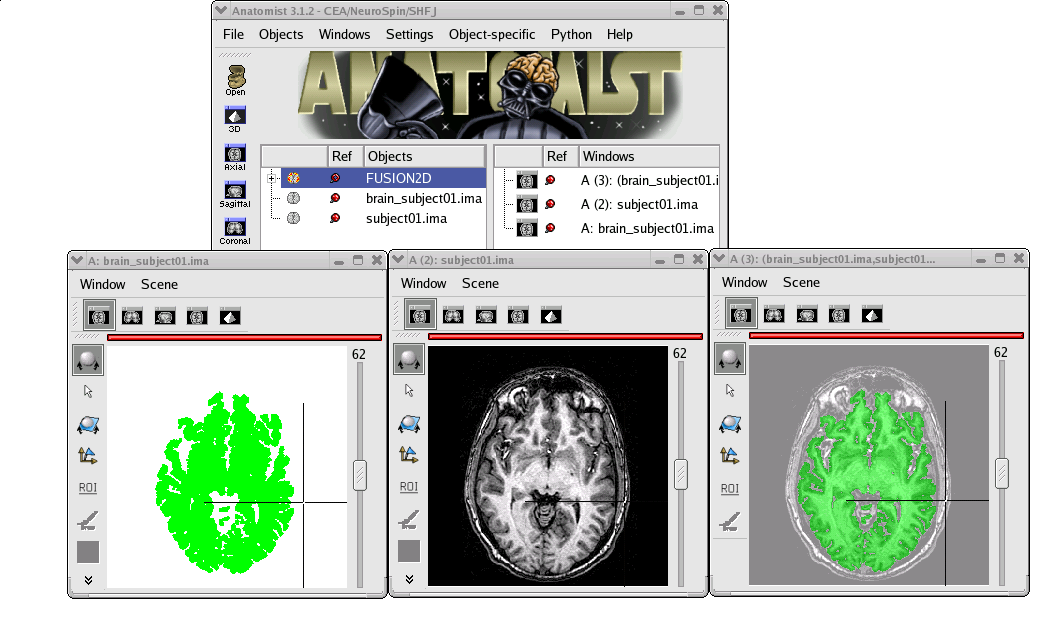
• STEP 1: Load the images to merge. Here, we will fusion an anatomy and the brain mask obtained from BrainVISA anatomical pipeline.

• STEP 2: Select the two volumes in objects list with Ctrl + left button.

• STEP 3: Then click on fusion button .

• STEP 4: A new window pop up to select objects order and fusion type (fusion types offered differs according to selected objects, this will be detailled later, in advanced part of the manual).

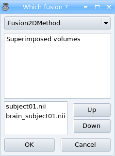
Fusion type

• STEP 5: Click on Ok to create the new Fusion2D object.

• STEP 6: Put the Fusion2D object in a window.

• STEP 7: If the Fusion2D object is all in black, you must change fusion mode. So right click on Fusion2D object to get its menu. Choose Fusion => Control 2D fusion. This window opens:

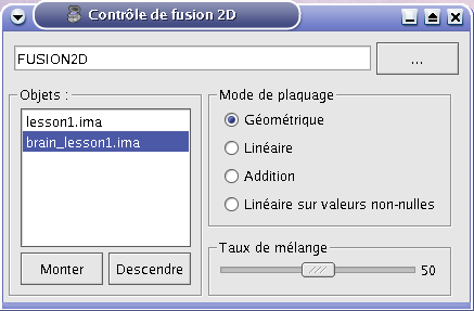
Fusion control

• STEP 8: You can change the mapping mode. The default is Linear: it does a linear combination of the two volumes. The Geometric mode does RGB channels multiplication. For linear fusions, you can set objects transparency with the cursor Mixing rate.

• STEP 9: By default, the 2 volumes will have the same palette. To change at least one, do Right clik menu on a volume => Color => Palette.

Example of a linear fusion between two 3D volumes

Note

It is possible to fusion more than 2 objects. For volumes, here is the method: with for example 3 volumes (V1, V2 and V3), Anatomist actually fusion the last volume and the volume above in the list (V2 and V3 gives V23). Then, from this fusion object, it creates a new fusion with the volume above (V23 and V1 gives V23_1). To set parameters for each fusion, you have to select the fusion’s second volume. For example, to set parameters for fusion V23_1, you must select V2.

Note

In this example, we did not have to matter about objects referential management because the brain mask (brain_lesson1.ima) have been generated from the anatomy, so objects are in the same referential. But if we had done a fusion between an anatomical volume and an activation map (which is in another referential since this map comes from a functional volume), we would have to handle referentials to put the objects in a coherent coordinates system.

Types of fusions

The following table shows the available types of fusion according to the type of objects. This list is extensible so all fusion types may not be in this list.

Fusion descriptions:

Objects	Fusion name	Description
Only one volume or 2D fusion	FusionSliceMethod	Fusion allowing to cut a volume across itself: to view/intersect 2 different slices of the same volume in the same window.
2 or more volumes	Fusion2DMethod	The volumes are merged in one volume. A voxel of the resulting volume is a combination of the same voxel in each original volume.
Volume + Mesh	Fusion3DMethod	Maps on the mesh a texture corrsponding to the volume values.
Mesh + (Volume or 2D fusion)	FusionCutMeshMethod	Mesh cut by a plane: the cutting plane will have the texture of the volume slice. When you put this object in a 3D window, the "cut mesh" control is available. It enables to control the orientation of the slice (shift) and its position (ctrl) against the mesh.
2 textures	FusionTextureMethod	Creates a 2D texture from two 1D textures.
Several textures	FusionMulitTextureMethod	Multi-texture: allows to map several textures on a mesh.
Mesh + Mesh	SurfaceMatcher	Matching surfaces. This object gives access to a surface deformation algorithm. It tries to transform one surface into the other.
Mesh + Texture	FusionTexSurfMethod	Textured surface.
Any object(s)	FusionClipMethod	Clipping: clips objects with a clipping plane. One side of the plane is cut and not displayed.
Volume or 2D fusion	FusionRGBAVolumeMethod	Converts an intensity-based volume (normally using a colormap) into a RGBA volume representation.
Volume or 2D fusion	VolumeRenderingFusionMethod	Displays a volumic object in 3D using intensities transparency on the whole volume.
Textured mesh + another mesh	Interpoler	Allows to map and interpolate textures from a mesh to another mesh with a different geometry. To obtain reasonable results, it is recommended to use a "SurfaceMatcher" first, it will warp a surface towards the other one
Mesh	Fusion2DMeshMethod	Marks the intersection line of a mesh with the view slice plane.
Volumes (1 to 3)	VectorFieldFusionMethod	(new in Anatomist 4.6) Vector field display: draw small lines at voxels locations showing the direction and intensity of a vector field. Vector components may be taken from a 4D (or more) volume, a RGB volume, or a combination of several volumes.
Normals	NormalsFusionMethod	(new in Anatomist 4.6) Display lines representing a mesh normals at each vertex position.

Fusion3D parameters

The 3D Fusion is a fusion between a volume and a mesh. This fusion can be parameterized through the right click menu on the fusion object.

You can change:

• Fusion mode: Geometrical, linear, rate.

• Methods of interpolation: the method to estimate the value for the intersection between the mesh and the volum at each point.

  Interpolation methods:

  Section	Description
  Point to point	the simplest: only the information coming from the voxel directly under the mesh vertex is used, directly. Do not use the depth and the step prameters.
  Point to point with depth offset (inside/outside)	Only one voxel is taken into account, but its position is shifted along the normal to the mesh (either inside the mesh or outside), for each mesh vertex (<Step> is not used here).
  Line to point	Information is taken along the normal line, both inside and outside, with a sampling (depth and step) specified by appropriate parameters.
  Inside line to point	The value corresponds to <the_choosen_submethod> value for the interpolation for a inside line localized at <Depth> and for a sampling <Step>
  Outside line to point	The value corresponds to <the_choosen_submethod> value for the interpolation for a ouside line localized at <Depth> and for a sampling <Step>
  Sphere to point	A sampling into a sphere (depth and step parameters apply) is used to get locations in the 3D volume

• Submethods: This only applies to interpolation methods that are not single-voxel (such as point to point methods)

  Interpolation sub-methods:

  Section	Description
  Max	The maximum value of all voxels of the volume at the sampled locations is mapped on the mesh
  Min	The minimun value of all voxels of the volume at the sampled locations is mapped on the mesh
  Mean	Standard mean (sum of values divided by the number of locations)
  Corrected mean	Only non-nul values are taken into account in the mean computation: this is more suitable for thresholded activation maps for instance to avoid blurring the mapped values.
  Enhanced mean	In the enhanced mean variant, a weighting of the final value is applied depending on the proportion of null values in the set of mixed values.

• Parameters: definition of localization of another point to do an interpolation

  Interpolation parameters:

  Section	Description
  Depth	Position of the other point
  Step	Sampling step. Always inferior to Depth.

Note

Be aware that all this is only a visualization toy and is not very robust: no real interpolation of the volume values is performed to get a continuous intersection along the mesh: especially the methods taking points along normals can produce inaccurate results on high curvature regions (produce discontinuities, map the same voxel value on several vertices etc). The sphere mode is more robust but involves an averaging (blurring) effet, and can take values outside the brain or grey matter…

About referentials

Load and display objects

Loading and displaying are two different actions in Anatomist. Loading is reading data stored in memory. While displaying is visualizing the object in Anatomist windows, with maybe modifications.

Axis orientation

Axes in native images in Anatomist are oriented like this:

• X axis: right => left

• Y axis: anterior => posterior

• Z axis: top => bottom

• T axis: 4th dimension to visualize a volume with an adding cursor to move from volume to volume; This axis can stand for the time in functional volumes vizualisation or directions for a diffusion sequence.

Neurological and radiological convention managing

Reading volumes on disk

When loading a volume, data organisation is supposed to match axis organisation describe before. That is to say data is loaded in radiological convention in memory (“LPI” convention, the contrary of the more used “RAS”).

Some image formats, however, do not specify correctly their voxels orientation without ambiguity. This is the case for the old ANALYZE format (almost disapeared, hopefully). Here, reading and displaying data depends on the following properties (attributes in .minf file and .aimsrc configuration file):

• Attributes spm_normalized and spm_radio_convention in .minf file of the volume (GIS format).

• .aimsrc configuration file of the user.

• .aimsrc configuration file of the site.

• .aimsrc configuration file of the package.

• By default, the SPM2 mode is used.

Note

If spm_radio_convention attribute value is 1, data in ANALYZE format is in radiological convention on disk. Else, if spm_radio_convention value is 0, data is in neurological convention.

See AIMS Configuration file .aimsrc.

What is SPM99 mode ?

We hope SPM99 is not used any longer thus this paragraph is obsolete.

The following explanations are valid only if your site / computer is configured as ours according to the flip parameter of SPM99. So for us, non normalized volumes are in radiological convention and volumes nomralized by SPM99 are in neurological convention. That’s why volumes identified as normalized volumes (according to their size in mm) are automatically flipped, to have a coherent display with data in radiological convention.

To go on working in SPM99 mode, your .aimsrc file must be configured like this:

attributes = {
    '__syntax__': 'aims_settings',
    'spm_input_radio_convention': 1,
    'spm_input_spm2_normalization': 0,
    'spm_output_radio_convention': 1,
    'spm_output_spm2_normalization': 0,
}

Volumes in analyze format are read in radiological convention ('spm_input_radio_convention': 1) and normalized volumes in neurological convention ('spm_input_spm2_normalization': 0).

Reading normalized volumes in SPM99 mode

As it is said before, in SPM99 mode, Aims tests the volume dimensions to see if it is normlized or not. A volume is considered as a normalized volume if its dimensions in mm are 152 < x < 165, 185 < y < 195, 130 < z < 145 or 178 < x < 185, 215 < y < 220, 178 < z < 185. In this case, the volume is supposed to be in neurological convention and it is automatically flipped at loading to display it in radiological convention.

What is SPM2 mode ?

We hope SPM2 is not used any longer thus this paragraph is obsolete. Later versions of SPM are using NIFTI or Minc image formats, which (when correctly used) do not present ambiguity.

It is different for volumes normalized with SPM2. Indeed, there is a parameter defaults.analyze.flip which indicates if input data must be flipped. (for more details, see SPM2 documentation). So data normalized with SPM2 can be either in radiological convention or in neurological convention. The aim is to keep the same convention for input and output data (before and after normalization).

To work in SPM2 mode (input convention = output convention), your .aimsrc file must be configured like this if your data is in radiological convention:

attributes = {
    '__syntax__': 'aims_settings',
    'spm_input_radio_convention': 1,
    'spm_input_spm2_normalization': 1,
    'spm_output_radio_convention': 1,
    'spm_output_spm2_normalization': 1,
}

Note

We will not deal with the case where input data is in radio convention and output data (normalized data) in neuro convention.

Anatomist needs make this kind of guess because there is no reliable information to indicate the convention in the Analyze format. Some header attributes have this information but it can be incorrect or out of date.

For this reason it is strongly recommended not to use the Analyze format, but to prefer more “modern” volume formats such as NIFTI.

Coordinates system

Definition

When loading any object (volume, mesh, ROI graph…), it has coordinates (in mm for meshes or objects with floating point coordinates, or in voxels for matrix-based objects like volumes, which also have voxel sizes to get to mm coordinates). An object thus has a “native” coordinates system, in which coordinates are directly expressed.

For volumes, Anatomist is using a native coordinates system referential in “LPI” convention (axes oriented toward (Left, Posterior, Inferior) of the head), the contrary of the more used “RAS” (Right, Anterior, Superior) as in MNI coordinates system.

Meshes may be in any native coordinates system, but unless specified in their header, Anatomist will think they are also in LPI orientation by default.

Anatomist manages transformations between referentials, which allows to display on-the-fly objects with transformed coordinates in a different referential.

Mecanism

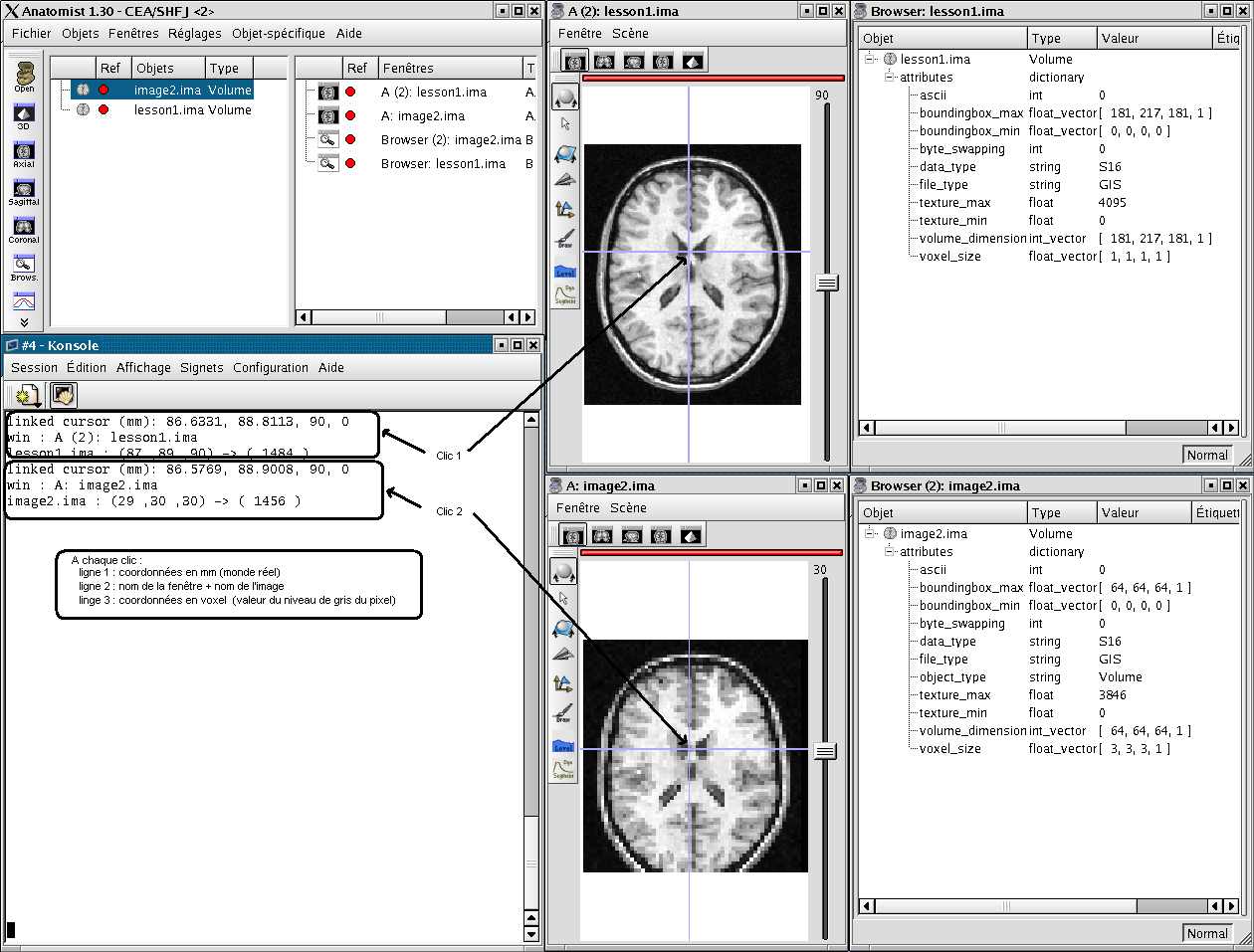
When you click on an object in a window, the position of the cursor appears in the terminal, and in the status bar of the window. This position is given in mm. After the position, you find the value of the voxel or of the texture, if any.

If the window contains several objects, the coordinates of each objects are displayed.

Coordinates in mm / coordinates in voxel

Coordinates systems

Coordinates is a matter of conventions. Conventions may (and actually do) differ between different software worlds. Anatomist (and the AIMS library underneath) is using certain conventions, and other software have taken different ones.

Anatomist is using for native image referentials a “LPI” system: axes oriented toward (Left, Posterior, Inferior) of the head. SPM and the MNI coordinates system are using the contrary, a “RAS” (Right, Anterior, Superior) system. For Anatomist it is certainly a bad choice, historically done about 25 years ago, because this referential is “indirect”, but whatever, it doesn’t forbid any functionality.

The origin of volumes, in their “native” coordinates system, is the “first” voxel in the corner of the volume. This voxel is located forward, on top and on the right of the volume. So, in an axial Anatomist window, this point will be at the top left corner if you keep the radiological display mode. The origin of the volume is the centre of this first voxel.

Anatomist manages affine transformations toward any other orientation. But such transformatons must be provided to Anatomist, it cannot (or not always) infer missing information.

Some objects (like NIFTI images) contain transformations toward other coordinates systems in their header. By default, Anatomist does not apply these transformations, because we don’t always know which are these referentials, and it could lead to errors (NIFTI is not very precise, it just has a code for “MNI”, “acquisition scanner coordinates”, or “other”).

In comparison, SPM and some other software do apply transformations by default, generally assuming that all loaded images have a transformation to a common referential. This assumption may be OK when all images have a transformation toward a norlmalized referential (MNI for instance), or are all images acquired in a single scan session where the scanner referential is actually the same. But in other situations, it’s wrong.

Anatomist can be asked to apply these transformations by default: it can be set in the preferences (volumes/use header information fore referentials/transformations) - don’t forget to save the preferences in your config if needed.

The preferences also allow to assume that all “scanner-based” coordinates system are the same (otherwise each imahe will have its own one with no connection to others). In the same preferences panel, check the appropriate option (and save if needed).

Once this is set Anatomist will try to make links between objects referentials, but will sometimes make wrong links.

Anyway ther is no miracle solution: there will be mistakes in links in inter-subject, inter-acquisition etc. But with these settings, Anatomist will behave “close” to the behaviour of SPM or other viewers.

The only reliable solution is to maintain a complete database of referentials and transformations. This is what BrainVISA does (https://brainvisa.info).

There are several coordinates systems (referentials) managed by Anatomist more or less automatically. That is to say some transformations can be loaded automatically either via BrainVISA, or by Anatomist. For example, if a volume is identified as a normalized volume (SPM), then the transformation toward SPM referential is loaded.

• Object referential: this is the real world sampled like explained before.

• Talairach-AC/PC-Anatomist referential: In BrainVISA Morphologist pipeline (T1 anatomical images segmentation), an affine transformation is computed: it is based on AC and PC points indicated by the user on the anatomy.

• Talairach-MNI template-SPM referential: Transformation applicated if the volume is normalized.

Note

Anatomist always loads a transformation from Talairach-AC/PC-Anatomist referential to Talairach-MNI template-SPM referential.

Coordinates systems and meshes

Meshes are handled the same way as other objects like volumes. However they are less constrained than volumes: mesh coordinates are floating point, and may be negative or positive (contrarily to volumes). Thus a mesh may have native coorinates in any coordinates system. It depends on how it has been built.

Typically, meshes built by Morphologist will have coordinates in the T1 MRI image native coordinates (an indirect referential), while meshes from Freesurfer will have coordinates in the MNI space (a direct referential). It’s then a matter of assigning them the right referential.

Until specified by the user, the mesh header, or an external program, Anatomist will think meshes are in an indirect referential.

Note

mesh in a wrong coordinates system

When a mesh is assigned a wrong coordinates system, it may appear symmetrized. This will typically make a left hemisphere mesh as a right one, and the contrary. This is tricky and important since it may lead the user to make mistakes (not speaking about flipped analyses). For instance between an individual volume referential (indirect) and the MNI space, all 3 axes should be inverted (the transformation matrix should have negative values around -1. on their 3 diagonal axes). If you load such a mesh in a software which does not have this transformation, then it will appear flipped (on all axes).

Another point with meshes is that they have a notion of interior / exterior, used for rendering and shading.

The exterior of a mesh is given by its polygon orientation (front_face property of the material or material entry in the object header: clockwise (normally in indirect referentials) or counterclockwise (in direct referentials).

Normals are used for lighting and shading, and should thus match the exterior notion.

In Anatomist (and generally in OpenGL) a mesh may be rendered in “single face” mode (only triangles seen from ther external side are drawn) or “double face”, so when there is an interior/exterior problem, meshes may be almost entirely not drawn (because most polygons are seen from the interior), and when there is a normals inversion issue, the mesh will be completely black because not lit at all.

A mesh may be transformed using a transformation in Anatomist, or externally, using the AimsApplyTransform command.

Linked cursor position

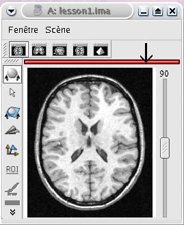
The linked cursor position is defined from the origin of the object. You can move the cursor to an exact position by fixing x, y, and z via the window menu: Scene => Manually specify linked cursor position. You can also use the shortcut Ctrl + P. You specify the coordinates in mm like this: x y z.

Referentials and transformations in Anatomist

General definition

A referential stands for a coordinates system and can be allocated to an object. So an object can moved from its referential to another if it exists a transformation between the two referentials. This transformation enables to change the corrdinates.

A referential can be allocated to an object or to a window. A transformation between two objects enables to align one object with the other. Whereas a transformation between an object and a window changes the point of view for visualizing the object.

Transformation format

Anatomist manages affine transformations: translation, rotation, zoom. It uses its own .trm format. It is an ASCII file, so it can be opened and modified with any text editor. It contains a 3x3 matrix and a translation vector.

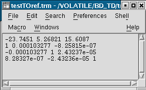
Example of a transformation .trm file

This means:

Tx	Ty	Tz
Rxx	Rxy	Rxz
Ryx	Ryy	Ryz
Rzx	Rzy	Rzz

This format defines a translation T and a rotation matrix R. Let R1 the refenential of a first volume and R2 the referential of a second volume. The file R1_TO_R2.trm specifies a transformation that moves from R1 to R2. So we have the following relation between coordinates of the two referentials: X2 = R *  X1 + T. This can also be written using a classical 4x4 matrix, where T is the 4th column.

The name of transformation file is generally *TO*.trm where each * is a referential. For example: refimage_TO_Talairach.trm. These transformations apply between two referentials and modifies only display of corresponding objects. Data on disk is not modified.

Referential of an object

Definition

Each object has an associated referential. Referentials are useful to compare objects. Without referentials each objects would be in its own coordinates system (sampling of the real world according to volume dimensions and voxels size) and objects coming from different modalities or acquisition would not be comparable. With identified referentials and transformations to move from one to another, it is possible to put objects in the same referentials in order to superimpose or merge them in a consistent way.

Why changing the referential of an object, and how ?

Why:

• Put an object in a new referential and load a transformation to another object in order to compare the two objects. For example, you have registered an fMRI to a T1 MRI and obtained a transformation file. You can use this transformation to visualize the two original images in a consistent way: put each object in a referential and load the transformation from fMRI referential to T1 MRI referential.

• Put a new object (o1) in the referential of another object (o2) which has already a transformation to the referential of a third object. In this case o1 and o2 are supposed to be in the same coordinate system. For example, o1 can be a mesh obtained from the anatomy o2.

How: Click on the object and select Referential => Load And then choose an existing referential or create a new one if needed.

Referential of a window

Definition

Each window is associated to a referential. This referential is used to visualize objects. If the referential of the window is different from the referential of the containing objects, it can change the point of view if there is a transformation between the two referentials.

Why changing the referential of a window, and how ?

Why: For example to see several anatomical MRI in the same referential, Talairach-AC/PC-Anatomist based on AC and PC points defined in the process Prepare subject of BrainVISA.

How:

• Click on the colored bar indicating the referential. See the figure below:

  

  Modifying the referential of a window (1)

• A new window opens and you can create a new referential or choose an existing one:

  

  Modifying the referential of a window (2)

Managing referentials and transformations

Most of the management is done using the Referentials window. To open it, use the menu Settings => Referential window.

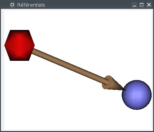
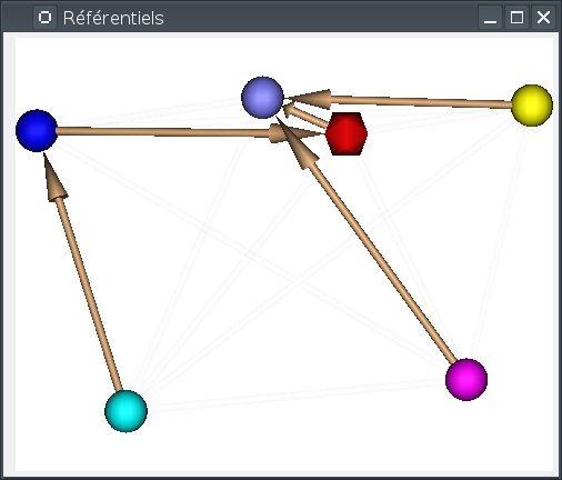
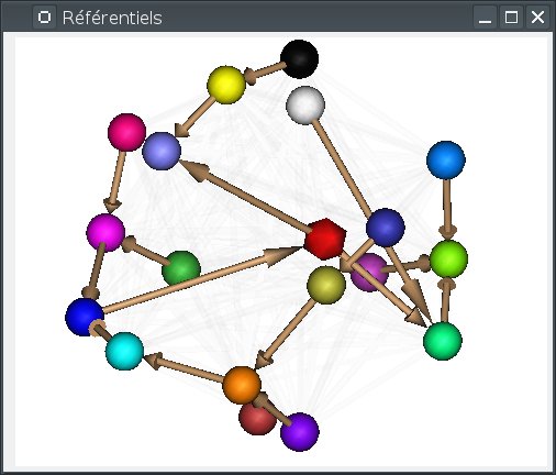
• In this window, referentials are displayed as colored spheres.

• Two special referentials are always present: the Talairach-AC/PC-Anatomist referential, whish is displayed as the red icosahedron, and the Talairach-MNI template-SPM referential, which is light blue.

• transformations are displayed as arrows joining the referential spheres.

• Implicit transformations (combining several explicit transformatons) are displayed in light.

The windows displays a 3D view with similar interactions as regular Anatomist 3D windows:

• the middle button rotates the view

• shift + middle button, or mouse wheel, controls the zoom

• control + middle button translates the view

• right button opens a popup menu

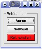
Anatomist older than 4.6 was using a 2D view with colored circles. This view is still present, it can be switched using the popup menu “legacy 2D view”, but the 3D view is likely to be clearer.

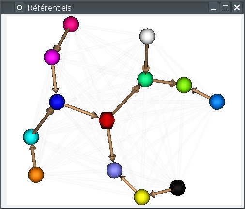
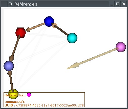
When the mouse gets over a referential (sphere) or a transformation, the corresponding object is highlighted, and information about it is displayed on an overlay on the window:

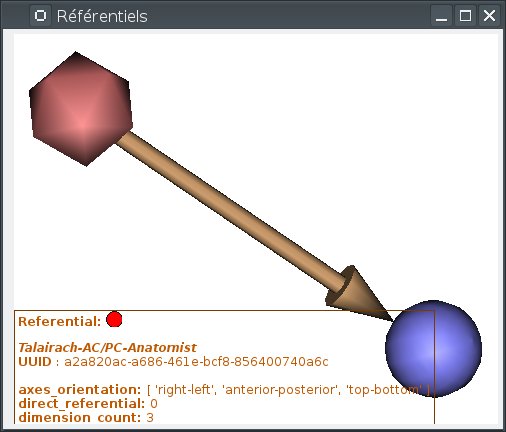
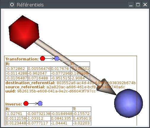
Info display can be toggled on or off by pressing the I key.

In this view, implicit transformations are present and are visible in very light colors: they can also display information and be used for interactions.

Interacting with referentials and transformations can be done in several ways:

• by using the popup menu while the mouse cursor is over the background: allows to create referentials, load transformations with referential information, clear unused or duplicate referentials…

• by using the popup menu while the mouse cursor is over a referential: allows to delete the referential, load its information, duplicate it, or show objects in this coordinates system.

• by using the popup menu while the mouse cursor is over a transformation: allows to delete the transformation, load a different transformation matrix, invert it, or merge the referenrtials linked by this transformation.

• by dragging with the mouse a link between two unlinked referentials: allows to load a new transformation from a .trm file.

• by dragging with the mouse and control key pressed, a link between two unlinked referentials: allows to create an identity transformation between two referentials.

• by dragging with the mouse and shift key pressed, a link between two referentials, either unlinked or linked by an identity transfortmation: allows to merge both referentials into a single one.

These actions are detailed a bit more below.

• When many referentials are present in the view, it is sometimes not so easy to distinguish all transformation arrows. It can be useful to rotate the view, or to rearrange the referentials positions. This can be done by pressing the F5 key. Referentials positions are taken randomly, then optimized by a placement algorithm which tries to limit arrows crossings for explicit transformations.

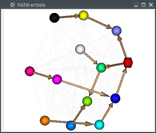
• Alternately the 3D view can arrange referentials on a “semi-flat” map (the default), or around a sphere. Switching between modes can be done using the background popup menu, or by pressing S (sphere) or F (flat). In sphere mode, F5 also rearranges the referentials positions around the sphere.

Loading a transformation between two referentials

To load a transformation between two referentials:

• open the referentials window

• To load the transformation, draw an arrow with the mouse from one referential to the other (take care of the direction). While dragging, a semi-transparent brown arrow will be drawn. If the mouse cursor gets over an incompatible referential (already linked to the source referential), the drawn arrow will become more transparent. Then a file dialog opens and you select the transformation file.

• Windows and objects associated to these referentials are updated.

Actions on transformations: delete, save…

The transformation menu is available by right click on the arrow representing the transformation (in the window Settings => Referential window). Here is this menu:

• Delete transformation: deletes the transformation between the two referentials.

• Invert transformation: inverts the direction of the transformation.

• Reload transformation: enables to change the transformation information by choosing a .trm file.

• Merge referentials: only enabled if the transformation is identity, in which case both referentials represent the same coordinates system, and can be merged into a single one.

• Save transformation: saves the transformation in a file. Used in transformation control (manual registration).

Creating an identity transformation between two referentials

In many cases we have to tell Anatomist that two distinct, existing, unlinked, referentials, are actually in the same coordinates system. We can draw an identity transformation between them.

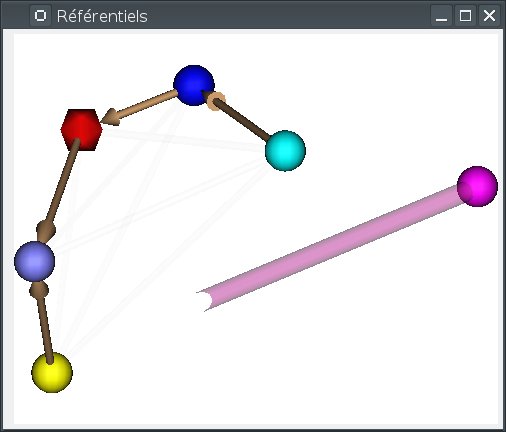
To do so, draw an arrow with the mouse from one referential to the other, while maintaining the Control key pressed. While dragging, a semi-transparent purple line will be drawn. If the mouse cursor gets over an incompatible referential (already linked to the source referential), the drawn line will become more transparent.

Merging two referentials

This can be done between two referentials which are not linked (neither directly nor indirectly), or which are linked by an identity transformation. This will tell Anatomist that both are in the same coordinates system, and that we will merge them into a single one. Transformations between them and other referentials will be preserved.

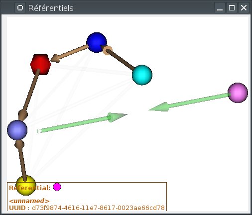
To do so, draw an arrow with the mouse from one referential to the other, while maintaining the Shift key pressed. While dragging, a semi-transparent green double-arrow will be drawn (it represents two referentials that will join together). If the mouse cursor gets over an incompatible referential (already linked to the source referential by a non-identity transformation), the drawn arrows will become more transparent.

Alternately, if an identity transformation already exists between the referentials to be merged, the merge action is also available on the right-click menu on the transformation.

Application: loading a transformation (coming from registration) between an anatomical volume and a functional volume.

For example, we want to visualize an antomical image (anat.nii) and a functional image (func.nii). We need to align the volumes using a transformation matrix (previously computed anatTOfunc.trm). Each volume has its own coordinates system.

• STEP 1: Load volumes, set a new referential for func.nii and create a linear fusion between anat.nii and func.nii.

• STEP 2: Select the menu Settings => Referential window.

• STEP 3: Then you see the referentials window.

• STEP 4: Draw a line with the mouse from one referential to the other according to the direction of the transformation. A file dialog will open.

• STEP 5: We can see that there is a now transformation between the two referentials and that the fusion display is updated.

Flash

Loading a transformation between an anatomical volume and a functional volume.

How to get a transformation file ?

There are several ways to get a .trm file:

• Using Aims commands to register 2 volumes (AimsMIRegister and AimsManualRegistration).

• Using Anatomist transformation control in order to do a manual registration.

• Convert SPM .mat files into .trm files using BrainVISA processes: fMRI => converters => SPM to AIMS transformation converter and fMRI => converters => SPM sn3d to AIMS transformation converter. Only the affine part of the transformation is converted.

• You can write your own transformation file.

Manual registration using Anatomist transformation control

Example: manual registration between a functional volume (Vf) and an anatomical volume (Va)

1. Load the volumes Va and Vf.

2. Fusion the 2 volumes to see their relative position.

3. Put the volume that have to be moved, Vf, in a window.

4. Select Vf in the window:

• Right click on the window

• Choose View / select objects

• select Vf in the browser window.</para>

5. In the window containing Vf, click on the transformation control.

6. You can move Vf in its window using the keyboard shortcuts.

NB: When you move Vf, a new referential is assigned to it. Indeed, Vf and Va are in two different referentials, and the transformation between these referentials is being computed.

NB: While you are moving Vf and Va, do not forget to look at all views: axial, coronal and sagittal.

7. Save the transformation:

• Settings -> Referential window

• The referential window opens. Each referential is represented by a colored round.

• Find the arrow betwenn Va and Vf referentials

• Right click on it and choose Save transformation

• Generally, the name is something like *TO*.trm, for example VfTOVa.trm

8. Edit the .trm file with a simple text editor to see the parameters of the transformation.

Using transformation information contained in SPM/NIFTI headers

SPM and NIFTI formats can store information about referentials and transformations in the header file. This information can be found in attributes spm_origin, referentials, transformations. It deals with referentials used in SPM. It can be useful to load these referentials and transformations when you have several images which are aligned in one of these referentials.

The Anatomist feature Load information from file header (in object menu => referential) loads the referentials and transformations mentionned in the header. If there is no transformation information, the feature does nothing. You can see the new referentials and transformations in the referentials window (in settings menu). The referential assigned to the object also changes. But by default, the display does not changes. Indeed, the default windows referential is Talairach AC/PC Anatomist and there is generally no link between this referential and the referential of the object. If there is a transformation between object’s referential and another referential and you change the window’s referential to this destination referential, the display will change.

If you set the user level to Expert, you can see another transformation when using Load information from file header: the transformation between the referential of the data on disk and the referential of the loaded object. This information is in the storage_to_memory attribute.

See also the tutorial

ROI drawing toolbox

Practical questions

What is the file format for ROI ?

Regions of interest are stored in a graph where each node is a ROI. Some attributes are associated to the graph and its nodes: the voxels size, name of each region… The file format is a couple .arg/.data. The .data is a directory and contains data of each region. The .arg is a file and contains the graph’s structure, that is to say nodes organisation.

It is also possible to export a ROI as a mask (a binary volume) using the option Region => Export as mask in ROI toolbox menu.

Accepted file formats to draw ROIs

You can draw ROI on 2D, 3D and 4D volumes.

How to open the ROI toolbox ?

You can either click on the icon in a window containing a volume, or press F1 key (obviously it will work only if there is a window containing a volume).

Some rules …

• A voxel cannot be in more than one region.

• You shouldn’t draw on a volume whose voxels size is different from the one of the graph. If it occurs, Anatomist will show a warning message.

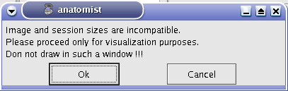
Warning message when volume and graph voxels size are different.

• Be careful to draw in a window which is in the same referential than the volume. Indeed, the voxels are drawn in the referential of the view, so if it is not the referential of the volume, the voxels of the ROI and the voxels of the volume won’t be in the same orientation.

ROI management interface

Here is the graphical user interface to manage ROIs:

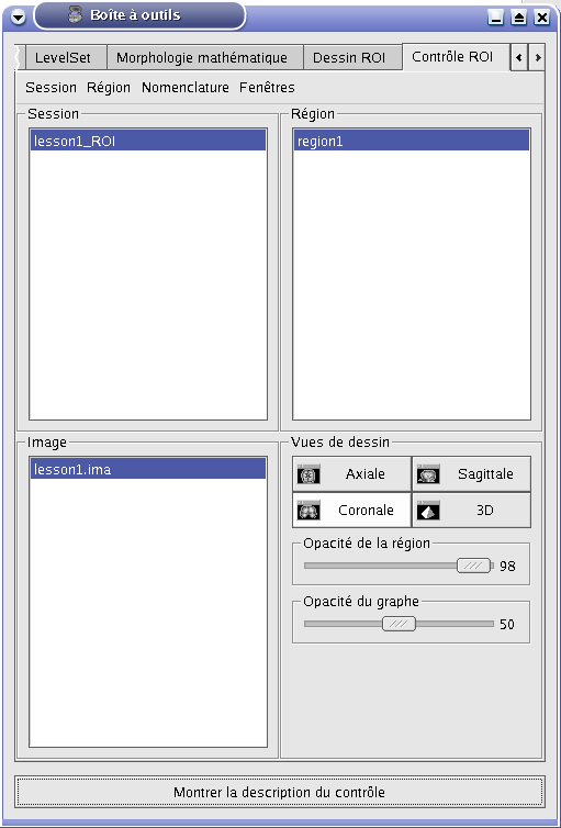
ROI management interface

Session menu

A session is actually a ROI graph. This menu enables to create a new graph, open an existing one, closing current graph…

Session menu:

Option	Description
New	Creates a new ROI graph. The default name is created according to the name of the selected volume in the Image panel. You can change the name of the graph using the Save as option.
Open	Loads a graph.
Close	Closes the selected graph.
Save	Saves the selected graph.
Save as	Saves and eventually renames the selected graph.
Clean	Deletes all isolated voxels. If you have drawn voxels by mistake, you can delete them using this option.

Region menu

This menu enables to manage the regions of the selected graph.

Region menu:

Option	Description
New	Creates a new region in the graph. The set of allowed names depends on the selected framework in the FrameWork option. If you want to choose your own names, use the Free framework (default). You can also load your own framework using the FrameWork => Personal => Load menu.
Delete	Deletes selected region.
Fusion	Merges several regions. The following window opens and you can select the regions that have to be merged and the name of the final region among selected regions names.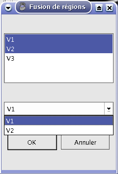
Export as a mask	Saves selected region as a binary mask (label volume).
Morphos Stats	Displays the volume in mm3 of the selected region in the console used to run Anatomist.

Framework menu

This menu manages nomenclatures used to name the regions.

Framework menu:

Option	Description
Neuro, Lateral Neuro, Sulci, Rat_wb	Pre-defined frameworks.
Personal	Enables to create and load custom nomenclatures.
Free	No selected nomencalture, each region name is given by the user.

Personal sub-menu

This menu manages custom nomenclatures.

Option	Description
New	Creates a new nomenclature for ROI graphs. First enter a name for the new nomenclature in a pop-up window. Then, a new object is created and shown in Anatomist main window. New sub-menus are available in the Personal menu: Define new region, Modify region name and Modify region color. One cannot define two nomenclatures at the same time. If you define a second nomenclature, you should save the first one, otherwise it will be deleted.
Load	Loads an existing nomenclature.
Save	The nomenclature is saved in the Anatomist config directory of the current user: <user_home_directory>/.anatomist/frameworks. You cannot choose the place to save the nomenclature.
Define new region	Sub-menu available on creating a new nomenclature. Enables to define a new region by giving its name and color.
Modify region name	Sub-menu available on creating a new nomenclature. Enables to modify the name of the current region.
Modify region color	Sub-menu available on creating a new nomenclature. Enables to modify the color of the current region.
Delete region name	This option enables to remove the current region from the nomenclature.

Windows menu

Windows menu:

Option	Description
Axial	Opens an axial window containing the volume and the ROI graph selected in image and session panels of the ROI toolbox window.
Sagittal	Opens a sagittal window containing the volume and the ROI graph selected in image and session panels of the ROI toolbox window.
Coronal	Opens a coronal window containing the volume and the ROI graph selected in image and session panels of the ROI toolbox window.
3D	Opens an 3D window containing the volume and the ROI graph selected in image and session panels of the ROI toolbox window.

ROI painting

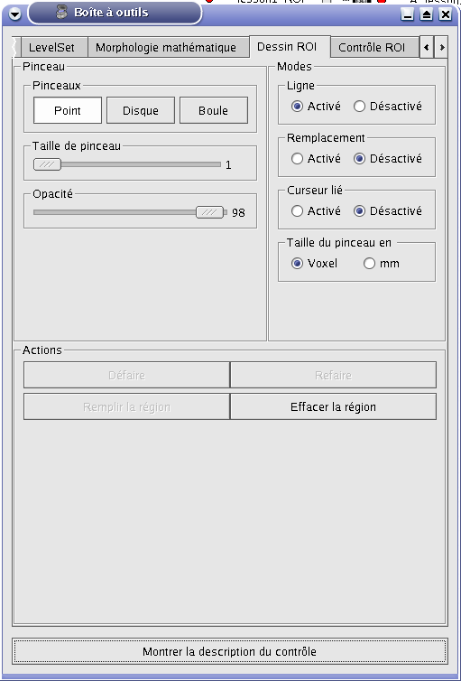
Paint tab

Brush panel

Brush panel:

Action	Description
Brush	Point: draw one voxel at a time. Disk: draw a “disk” within a radius of the “brush radius” size on one slice at a time. Ball: draw a sphere within a radius of the “brush radius” size on several slices.
Brush radius	Brush size in voxel or mm according to the chosen option in the Modes panel
Opacity	Sets the opacity of drawn ROIs. Decrease it to increase transparency.

Modes panel

Modes panel:

Action	Description
Line	On: outlines that you draw will be continuous even if you draw rapidly. Off: if you draw rapidly, lines will not be continuous.
Replace	On: Each voxel on which you draw will be added to the current region, even if it was already in another region. For examle, if a voxel V is in a region A and you are drawing a region B passing on voxel V, this voxel will move to region B. Off: a voxel which is already in a region cannot be put in another one.
LinkedCursor	On: you can see your ROI in several views simultaneously while drawing. Off: you cannot see your ROI in several views simultaneously while drawing.
BrushUnit	Voxel: the unit for the brush radius size is the voxel. mm: the unit for the brush radius size is the mm.

Mathematical morphology

This tab offers basic tools for mathematical morphology: operations (dilation, erosion…) realized on selected ROIs. You can choose the structuring element radius in voxels or in mm and realize 4 types of actions: erosion, dilatation, opening, closure.

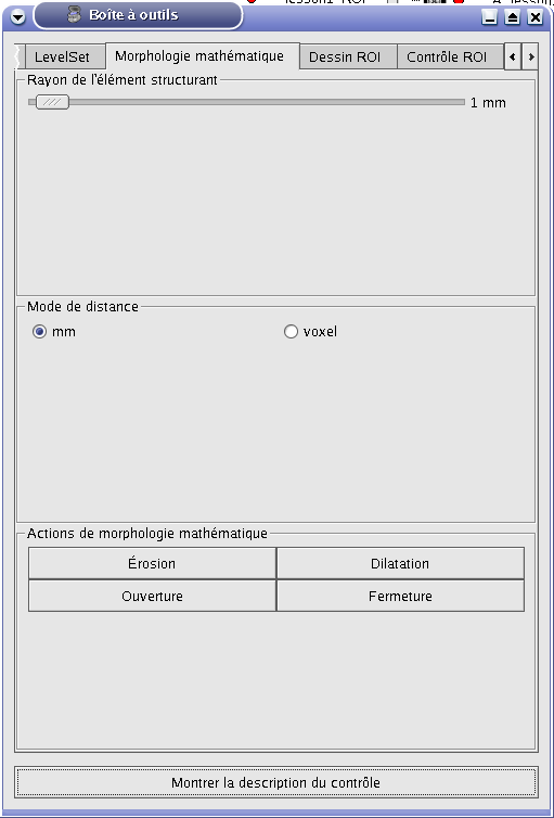
Mathematical morphology tab

Structuring element radius:

Action	Description
Structuring element radius	The structuring element is a shape composed of a set of points. The center of the element is applied in each voxel of the ROI. Here, the structuring element is a neighbourhood with a 6-connectivity.

Distance mode:

Action	Description
mm	The structuring element radius is in mm.
voxel	The structuring element radius is in voxels.

Mathematical morphology actions:

Action	Description
Dilation	Outline erosion: if the structuring element placed in a point of the ROI has an intersection with the volume outside the ROI, these intersection points are added to the ROI.
Erosion	Outline dilatation: if the structuring element placed in a point of the ROI has an intersection with the volume outside the ROI, this point is removed from the ROI.
Opening	Erosion then dilatation. This action enables to remove some little isolated regions, to smooth outline and to separate objects weakly linked.
Closing	Dilatation then erosion. This action enables to remove some little holes and to connect objects.

Connectivity threshold

This module enables to make a semi-automatic segmentation of a volume. You define a band of gray levels by selecting a low level threshold and high level threshold. Corresponding regions are highlighted and added to current region when you click on them. You can also export this region as a mask.

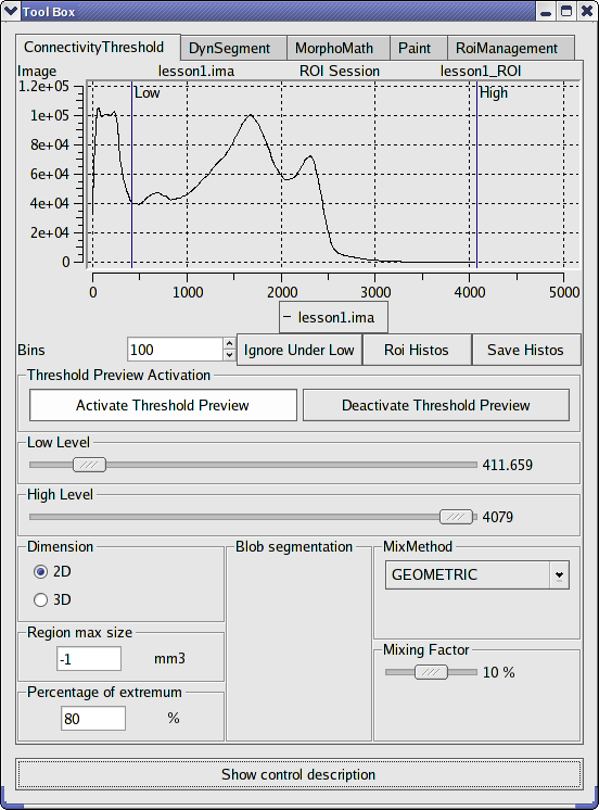
Connectivity threshold tab

At the the histogram of the volume is displayed: the y coordinate is the frequency of a gray level and the x coordinate is its value.

Connectivity threshold panel:

Field name	Description
Bins	Number of bins splitting the gray levels scale.
Ingnore under low	This option enables to update the frequencies of gray levels in the histogram according to the values of high level and low level.
Histo Image / Histo ROI	Histo Image: show the histogram of the volume for which connectivity threshold is activated. Histo ROI: show the histogram of each ROI of the selected graph.
Save Histos	Save all histograms (volume and ROIs histograms) in a text file. The format of this file is .anahis. The extension is optional and the file is readable with any text editor. See appendix anahis format
Activate threshold preview	Activate threshold preview: enable this option. If this button is not on, none of the other action is available. Deactivate threshold preview: disable this option.
Low level	Move the cursor to set the low threshold of gray levels.
High level	Move the cursor to set the high threshold of gray levels.
Dimension	2D: the region will be a 2D volume, it will be only in the selected slice. 3D: the region will be a 3D volume.
Mix method	Geometric: geometric fusion between the volume and the region defined by the threshold. Linear: linear fusion between the volume and the region defined by the threshold.
Mixing factor	Mixing factor used for the linear fusion.

Blob segmentation

In a PET exam, you can use this module in order to isolate a region according to a local maximum. A blob is a region around a minimum or a maximum. Here is the steps of this segmentation:

• Click on a point with Shift + left button near an extremum.

• The algorithm searches for the closest maximum.

• From this maximum, the region grows under 2 conditions: * the region size must not exceed the maximum size given by the field region max size (in mm3). * the values must not be lower than the threshold given in the field percentage of extremum.

• When the segmentation is over, the region is displayed.

• NB: it can occur that the region does not contain the original voxel; in this case a warning message indicates that you have to click closer.

Blob segmentation:

Field name	Description
Region max size	Maximum volume for the blob in mm3. For example, if the voxel resolution is 4x4x4 mm (the volume of a voxel is 64mm3) and you set 1280 mm3, the region size is 20 voxels.
Percentage of extremum	Percentage of the maximum value. It is possible to change between a maximum and a minimum using keys Shift+B (to a maximum) and Control+B (to a minimun).

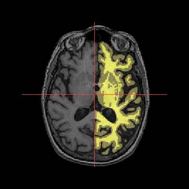
ROI drawing mode by label selection

Some volumes are called image of labels, that is to say each part/structure of the volume is identified by a voxel value: a numerical label. For example, in the following image, the volume contains the background, the left and right hemispheres and the cerebellum. And each part is associated to a label: voxels have value 1 in the left hemisphere, 2 in the right hemisphere, and 3 in the cerebellum.

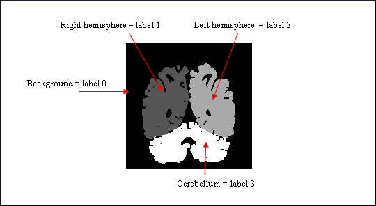
Image of labels (displayed in radiological convention)

With this control, you can select regions according to a label. For example, if a volume V has the labels: 1, 2 and 3:

• Load the volume V in Anatomist.

• Put it in a window and click on the ROI control.

• Create a ROI graph G and a region R to store your selection.

• In the window containing the volume V and the graph G, click on the label selection control .

• Click on a voxel which value is the required label.

• A warning message appears if the data is huge, click on yes to go on.

• You will see better your region in a 3D window.

• The region R of the graph G now contains the selected region. You can store this ROI graph or export this region as a mask to get a volume.

• NB: in advanced use, you can substract sub-regions using the control options.

Surface paint module

A surface painting module is present in Anatomist. This tool allows to draw textures on a mesh, using several drawing tools. This module has been primarily developed in the specific aim of drawing sulcal constraints to build a 2D coordinates system on the brain (see the Cortical Surface toolbox in BrainVisa), but can be used in a general way to draw any texture values.

To use this module:

• Load a mesh.

• Select it and click on in Anatomist main window.

• Click on the Ok button on the new popup window. The options in this window are useful only to build a 2D coordinates system on the cortical surface.

• A new 3D window containing the mesh opens.

• A new control should be available in the 3D window. Select it.

• Several new icons and parameters are now available in the 3D window to allow drawing on the surface.

The following table shows the meaning of the buttons and actions in this tool:

Surface paint module actions:

Action	Description
	Manual drawing on the mesh (unconstrained).
	Texture value picking tool. Click on the mesh to select the texture value at the selected position. This value will be used in later drawing operations.
	Erase a drawing. Restores the initial texture values at erased positions.
	Fill a closed region. The points included in the region are computed and shown to the user who must validate the drawing. A tolerance may be set to adjust the selected region boundaries on continuous floating point textures.
	Draw the shortest path between 2 points. The tool suggests a path that must be validated with .
	Draw with anatomical constraints. The drawing path is computed trying to follow the depth of the sulci.
	Draw with anatomical constraints. The drawing path is computed trying to follow the top of the gyri.
	Magic brush. Draws on the mesh, in the same way as the draw tool, but draws continuous lines by adding junction segments as needed.
	Validate a drawing suggested by an automatic tool like the magic wand or the constrained paths.
	Cancel a drawing suggested by an automatic tool like the magic wand or the constrained paths.
	Distance maps tool. Click on the mesh: it will fills the texture with the geodesic distance to the click point position.
	Undo the last action, which may be either a fully validated action (complete path, fill, brush stroke), or the last unvalidated action in a compound action (last control point in a curve…)
	Redo the last undone action (or sub-action, see undo above).
	Save the drawing in a texture file.
Texture value	Change the current texture value used to draw on the mesh.
Tolerance	Determines the tolerance of the magic wand tool selection values.
Tension	Changes the smoothness of curves drawn by the geodesic path tools (with constraints).

In addition to these tool buttons, and as in other Anatomist controls, several keyboard and mouse shortcuts are available in the surface paint mode: see the SurfPaint control description

See also the Surface paint module tutorial

Handling a graph

As we saw before, graphs enable to represent structured data with nodes and associated attributes. Graphs also have global attributes defining characteristics shared by all nodes, as for example voxels size. Nodes also can be linked by relations. This is used in sulci graphs to represent several units extracted from a sulcus. You can see these relations by selecting the neighbours of a node.

Graph nodes contain structures labels (for sulci and ROI graphs), which may be stored in two possible attributes, name and label. These two attributes have the same role: naming a node. Then, it is possible to make a link with a nomenclature file in order to associate a color to each value of attributes name or label.

So, what’s the use of having two different attributes with the same role ? In some cases, we need a double identification. For example, in a automatic sulci recognition, nodes are renamed by computer experts. When consulting the results, you might want to rename a sulcus and keep the original identification, which is highly recommended.

Browsing a graph through its nodes

Follow these steps:

• Put the graph in a 3D window.

• Right click on the window and select the menu View / select objects. A browser window opens.

• Then, you can select a node in the browser window, it will be highlighted in the 3D window.

• Conversely, when the selection control is active in a 3D window, clicking on a node in the 3D view will select it, both in 3D views and in browser windows. See next section for details.

If you do not want to see all the nodes of the graph because it is a big graph and you want to see only chosen nodes, you can use the object menu Display => Add without nodes available by right clicking on the graph. Select a window and use this feature, the graph will be loaded in the window but its nodes will not be visible. If there is no open window, Anatomist will open a new 3D window and load the graph in it. If there are several windows and none is selected, Anatomist will load the graph in each window. Then, you can use the menu View / select objects to select the nodes you want to see.

Selecting nodes

• Move to selection mode by clicking on the selection control of the 3D window containing the graph.

• Then you can select visible nodes clicking on them. The selected node change color in the 3D window and become selected also in the corresponding browser window. You can select several nodes keeping ctrl key pressed.

• You can also select neighbours of a node by choosing select neighbours in right-click menu. A node has neighbours when there are relations between the nodes. So you can select neighbours in a sulci graph where such relations exist, but generally not in ROI graph because there’s no link between different regions.

• You can undo selection by choosing unselect in right-click menu. This feature undo selection for all nodes currently selected. These nodes retrieve their original color.

• Finally, it is possible to remove nodes from the window by selecting them and choosing remove from this window in the right-click menu.

Graph parameters

The graph parameters configuration window is available through: Settings => Graph parameters

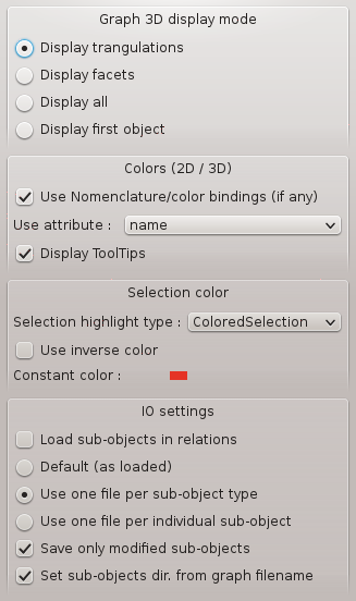
Graph parameters window

Graph 3D display mode

• Display triangulations: object surface is smoothed.

• Display facets: display “voxels”.

• Display: display both smoothed surface and voxels.

• Display first object: nodes in a graph can be made up of several objects that can be displayed by Anatomist. For example, in a sulci graph, nodes are made up of 4 displayable objects: 3 buckets (voxels lists) and 1 mesh. By choosing this option, only the first of these objects is displayed for each node. In a sulci graph, the first object is the mesh representing the sulcus.

Colors (2D / 3D)

• Use Nomenclature/color bindings (if any): enables to link attributes of the loaded nomenclature and of the loaded graphs.

• Use attribute Label/name: nomenclatures and graphs are linked through Label or Name attribute.

• Display Tooltips: display information tooltips when the mouse passes on objects.

Selection color

• Use inverse color: the color of the object is inverted when it is selected.

• Constant color: the color of selected objects is always the same. You can change it by clicking on the colored square.

IO saving settings

• Default (as loaded)

• Use one file per sub-object type

• Use one file per individual sub-object

• Save only modified sub-objects

• Set sub-objects dir. from graph filename

Using nomenclatures

Using a nomenclature file (icon: ) offers another way to browse a graph. For example, you load 2 labelled sulci graphs and the nomenclature of sulci recognition. Then you can select a sulcus by choosing its name in the nomenclature. So the choosen sulcus is displayed in each graph window.

Using a nomenclature also enables to associate a color to a label and/or a name. Thus you can standardize the display of graphs. A specific label or name will be displayed with the same color in every graph.

A nomenclature file has the .hie extension and is a simple text file. <para>Handle a nomenclature:

• Put the nomenclature in a browser window.

• You can now select nodes in graphs by clicking on the nomenclature’s nodes. It is organized hierarchically. This means that you can select all the graph nodes that are under a nomenclature name by clicking on this name. For example, if you click on the name of a lobe, all sulci in this lobe become selected. And when you click on “brain” in a sulci nomenclature, all identified sulci become selected (but not thosewith the label “unknown”). It makes it easy to visualize and select things by region.

Note

Simple nomenclature files for ROIs can be created using Nomenclature => Personal menu in the ROIs module in Anatomist.

Note

The nomenclature must match the graph type: value of graph_syntax attribute in the nomenclature must match the Value column displayed for the graph in a browser window (eg: “CorticalFoldArg” for a sulci graph).

Modifying the value of graph attributes and saving a new graph

You may need to modify some attributes values in a graph. For example, when you check sulci automatic recognition in a sulci graph obtained through a BrainVISA process. Indeed, during this process, each recognized sulcus is labelled using label attribute. Then, when you check the recognition, you can use the name attribute as a validation. Using the two attributes label and name enables to keep the automatic labelling and your manual labelling.

Modifying the name attribute in a node and recording a new graph:

• Load the graph.

• Put the graph in a browser window.

• Unroll the node you want to modify.

• Go to the name attribute.

• Right click on it to display a menu.

• Choose Modify attribute.

• Type a new value for the attribute.

• When all modifications are done, go to the graph in Anatomist list of objets in the main window (left panel).

• Right click on the graph and choose File => Save in order to save the graph with the modifications. You can choose a new name or to keep the same but in this case the original graph will be erased.

Anatomist surface matching module

Surface matcher

This module allows to drive the deformation of a mesh towards another. It was written originally to be used for EEG applications, where the EEG model (generally a sphere) needed to be matched to the subject head to get the coordinates of EEG electrodes.

• Load 2 meshes in Anatomist

• Perform a fusion of both meshes, using the “Surface matcher” mode. This results in a new SurfMatch object.

• Select this SurfMatch object contol panel via the right-click menu Object manipulations => Fusion =>Surface matching window.

• Open the SurfMatch obect tree. It contains 3 children objects:

  • the two initial surfaces

  • a new mesh: matchsurf.mesh. This one will be the mesh actually deforming.

• Open a 3D window

• Put the target surface and the matchsurf.mesh mesh in the window. At the beginning, the deforming surface os not visible (it is uninitialized, and empty).

Surface matcher control window. Note the antique anatomist 1.17 graphical interface… The module has not changed a lot since this age…

• select the transformation direction in the surface matching window using the Change button

• Click on Reset: the deforming surface appears, and is identical to the source mesh.

• To see a bit more clearly, it may be useful to set different color materials to the 3 meshes, and some transparency on the target mesh (decrease the alpha coef of the diffuse material).

• Set the matching parameters in the central column, Matching parameters.

• If needed, add some control points: pairs of points directly attracted between both surfaces.

• the Record over time option allows to keep the whole iterative deformation sequence in the matchsurf.mesh mesh, in a time sequence. The sequence can be saved on disk as a regular mesh (it contains a timestep cursor). Warning: it may require quite much memory since all deformed mesh steps are kept in memory, especially if the source mesh contains many vertices/polygons.

• When everything is setup, the matching begins by clicking the Start button.

• It is possible to interactively change matching parameters, and to add or remove control points while the deformation is still processing: changes will be taken into account at the next processing step.

• When the user is OK with the result, processing can be stopped with the Stop button. Note that the processing will not stop on its own: there is no convergence criterion.

A deformed mesh has the same topology as the source mesh: same number of vertices and polygons, in the same order. Just the position of vertices have changed (to fit the destination mesh). Thus one can map textures suitable for the source mesh on the deformed one:

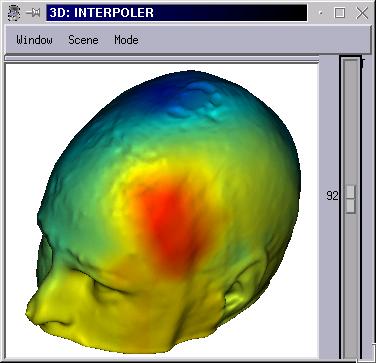
Intepolation of functional data from one surface to another

This interpolation is meant to map texture data on a mesh which is finer than the mesh it is normally associated with. Typically, map EEG data acquired on a set of electodes locations (generally 64, 128 or 256) on a head mesh with several thousands of vertices.

To work properly, the ineterpolation should use two “registered” meshes: the source mesh should be deformed to match the destination mesh geometry, which is typically done using the Surface Matcher feature.

If the matching has not been done, the interpolation will probably produce erratic and ugly results.

• Load both meshes

• Load the texture for the source mesh (functional data)

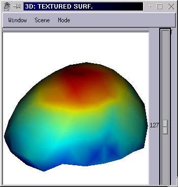
• Build a Textured Surface fusion between the source mesh and the functional texture (ie EEG electrodes net mesh, deformed to match the subject head, and EEG data)

• Make a second fusion between the textured surface (1st fusion) and the target mesh (ie head mesh). Select Interpoler mode.

• Put this Interpoler object in a 3D window, and change its palette

The interpolation is a linear one (fast and simple).

Interpolation takes place on the fly, time slider actions may be slower than on a regular texture.

Appendix: anatomist command options

[ -i | --input <vector of string>]  loads these files (conataining either Anatomist/AIMS objects, or .ana commands files)
[ -p | --pipe <vector of string>]   open named pipe to read commands from (differs from normal .ana files loading in that the pipe is not closed once read,
  the pipe is reopened once flushed - using -p for a regular file results in infinite rereading of the same commands file)
[ -b | --batch <boolean>]  batch mode: no control window (for remote control only, normally used with -p or a .ana input)
[ -s | --server <S32>]  server mode: anatomist will listen on the given TCP port for command stream connections
[ -u | --userprofile <string>]  user profile: all personal data will use the directory<home_dir>/.anatomist-<userprofile> rather than
  the default<home_dir>/.anatomist
[ --enable-unstable <boolean>]  Enables unstable features which may make Anatomist badly crash (experts only) (and nobody could tell you which features this incudes)
[ --cout <string>]        redirect outpout messages to a file
[ --cerr <string>]        redirect error messages to a file
[ --verbose [ <S32>]]     Set verbosity level (default = 0, without value = 1)
[ -h | --help <boolean>]  show help message
[ --version <boolean>]    show Cartograph version
[ --info <boolean>]       show libraries information (install, plugins, paths, etc.)

Appendix: Loading convention according to Aims version

Guesses for Analyze format images

Aims version older than 2.13

Non-normalized images were read in radiological convention and displayed according to Anatomist configuration.

Normalized images were read in neurological convention because of SPM 99. Indeed, SPM 99 always write normalized images in neurological convention.

Aims version >= 2.13

Since this version, normalized images are managed differently by Anatomist because of SPM 2. Indeed, images normalized with SPM2 can be in radiological or neurological convention, it depends on the source image. The output image keep the convention of the input image.

So by default, Anatomist loads and displays images in radiological convention.

A configuration file enables to modify theses loading and displaying parameter for a site or a user. For more details, see AIMS Configuration file.

Anatomist script files (.ana)

All actions done in Anatomist interface are stored in a file history.ana in your .anatomist directory (in C:Documents and Settingsuser_name under windows and /home/user_name under linux). You can save and reload this script to retrieve rapidly a session. When your session is ready (objects loaded, windows opened…), you have to save the history.ana by changing its name or copying it in another place else it will be erased the next time you start Anatomist. When you want to reload the session, start Anatomist using the anatomist command with the script filename as a parameter. For example:

anatomist /tmp/history.ana

You can also load a script file by using the menu File => Replay scenario.

More on colors and palettes

Adding a new palette

• Go into your .anatomist directory. It is C:\Documents and Settings\user_name\.anatomist under windows and /home/user_name/.anatomist under Unix.

• Create a directory rgb if it doesn’t exist yet.

• Put the palette files in it. It can be for example in GIS or JPG format, or any image/volume format readable by Anatomist.

• This new palette will be available in the list of palettes in Anatomist when Anatomist is restarted. If it is aleady running, use the menu Settings => Reload palettes.

Details on how palettes are working

Palettes and opacity

Textures may be using RGB or RGBA values or palettes. Transformed palettes color are then mapped onto a mesh, using a given “blending” mode.

Volumes are similar to textures, because in Anatomist a volume slice is a square mesh in 3D space with a texture on it.

It is thus possible to tweak both the RGBA palette (with or without opacity), and the mapping mode (texturing properties).

Texture

By default a mesh is opaque. The palette transparency (in RGBA mode) means the opacity of the texture in the blending with the mesh color (its material). It will not make the mesh transparent. The mesh transparency, in turn, is only given by its material (the “diffuse” part mainly).

The texture blending mode can be changed, in Anatomist interface, via the right-click menu on objects “color/texture”, or in a program via the TexturingParams command.

Volumes are using by default the decal mode (modes are defined in OpenGL).

If we want a semi-transparent mesh where its opacity is given by the texture, then we may use the geometric mode (geometric blending between the material and lighting, and the texture), or the replace mode (material and lighting are not taken into account any longer).

With several images

Stricto sensu, when there are several images in the same view, there are several squares in space, at the same location. The resulting rendering is not good: only one image will be seen, or it will be an aliased alternance between them (due to numerical imprecisions in OpenGL Z buffer). In order to get the expected result, images must be mixed (blended, or often called “overlayed”, but we have not used this terminology in Anatomist). In Anatomist we use a “fusion” of the images (2 or more) in a “Fusion 2D” object.

Anatomist (since version 4.6.1) build this 2D fusion automatically and internally; but as it is automatic, the user does not get (or not easily) full control over it. If you need to tweak it, it’s probably easier to build the fusion “by hand” (or in a custom application program code).

To be clear, the Fusion2D builds a texture resulting from the different images, then maps it on the square mesh (like for a single image). The way an image is mixed with another is determined by texturing modes and options, for texture indices >= 1. Texturing index 0 is the mapping of the final texture on the mesh.

Things should be seen the reverse way. Order is important. For instance if we have 3 volumes, A, B and C,

• Texture properties index 2 tells how to mix volume B with volume C.

• Texture properties index 1 tells how to mix volume A with the previous one (BC mix) etc.

• Texture properties index 0 tells how to map the result (ABC) onto the mesh.

For indices >= 1 (mixing between volumes) there are more modes than the OpenGL modes (it’s not an OpenGL multitexturing, Anatomist is making the mixing here, thus we have more flexibility). Some modes consider white or black colors as transparent, others are using the RGBA palettes. The mixing rate tells how to blend textures between the condidered layers (as described above). Remember that this mixing happens in RGBA space (after applying palettes), not in image values space.

Example

Let’s take a classical example with 2 images, say one anatomical MRI (we call it mri) and a labels image containing segmented objects (we call it seg). seg has the value 0 in its background, which we wish to be transparent.

We fusion (mri, seg), in this order (order can be checked and changed in the GUI in the Fusion2D object properties).

We set the “B-W LINEAR” palette on mri (gray levels, classical, this is the defaut).

We set a colored palette on seg. Let’s take one with a black color as 1st value (ex: “Blue-Green-Red-Yellow”). The background of this image is thus black:

We set the texturing mode for texture 1 of the fusion object (so: mixing between the two images mri and seg). Let’s use the mode linear_A_if_B_black (here A is mri and B is seg): where seg is black (background) we want to fully see mri behind.

Then the mixing rate sets the relative weight of mri and seg in the regions where seg is not black. If we set it to zero, the weight of mri is null, and we see only seg. Inversely if we set it to 1, we don’t see seg anymore:

If we had used for seg a palette wich first color is white (ex: “Blue-Red-fusion”), then its background would be white. We would rather have used the linear_A_if_B_white mode:

In both cases the resulting object (the 2D fusion) is opaque (black opaque background): if there is for instance an additional mesh in the view, we don’t see the parts behind the square of the 2D slice.

Now if we want the slice object to be transparent, we will use a RGBA palette for the mri object: for instance the “B-W LINEAR-transparent” palette. This specific palette is mostly opaque, except for the first color which is totally transparent. The lowest value of the image (0 generally) will thus be transparent. As there is generally noise in the image, the user will probably need to slightly increase the min value of the palette settings so that values under this threshold become transparent. But for not the slice object (2d fusion) is still not transparent: for this we also need to set the mixing mode between the final texture (mixed mri and seg) and the mesh. This is what the properties for texture 0 of the fusion object do. By default it is in decal (opaque) mode:

We can set it to replace mode (total replacement of the mesh material: the mesh colors and lighting do not apply any longer), or to geometric mode (multiplicative blend between the mesh material and lighting and the texture: lighting applies, the image becomes black when seen and lit from the profile side):

We could also use a semi-transparent palette for mri, like “semitransparent” or “semitransparent2” to get partial transparency on the mri object. Here we use “semitransparent” (both gray levels and opacity corresponding to the the image intensity) with a white background, and “semitransparent2” (all white, with opacity corresponding to the image intensity). Of course here, as objects are transparent and their color will mix with the window backgorund color, the window background color is important:

Objects properties used at load time

When loading objects, the reading system loads any supported format file, then tries to read an additional .minf file, which is specific to the Anatomist/Aims/BrainVISA framework. This additional file is text-based and may contain a set of properties to be added to the loaded object. Some properties may carry information which does not fit in all file formats (like image properties, diffusion information), coordinates systems specification, or any additional property.

The .minf format may be “python dictionary” (similar to json), or XML.

Some of these properties are interpreted by Anatomist, and may bring information with objects.

Property:	Applies to:	Description:
referential	all geometrical objects	referential identifier. The referential property is the one used directly for the object coordinates system. It may be a string identifier for a known referential, or an UUID (unique identifier), with the shape “9a839283-7642-d21a-f67a-836a205be5e3” for instance. Referential identifiers may be used in transformations to handle coordinates systems. String identifiers refer to “standard” referentials, and are mostly derived from the NIFTI referentials identifiers: “Scanner-based anatomical coordinates”, “Talairach-MNI template-SPM”, “Talairach-AC/PC-Anatomist”, “Talairach”, “Coordinates aligned to another file or to anatomical truth”.
referentials	all geometrical objects	|referentials_prop_doc|
transformations	all geometrical objects	A list of affine transformation matrices. Each of them transforms from the object referential (see the “referential” property) to another referential listed in the “referentials” property. Each transformation is given as a list of affine matrix (4x4) coefficients: 16 numbers, the matrix is written as lines.
palette	textured objects	A dictionary of palette properties. These properties have the same syntax as the SetObjectPalette command. In addition, in Anatomist 4.5 and later, palette properties can include additional information to define new, personal, palettes: colors: list of R, G, B or R, G, B, A values, all in one line, int values between 0 and 255. Depending on the “color_mode” property, values will be grouped by 3 or 4 to form colors. color_mode: “RGB” or “rgb”, “RGBA” or “rgba”: tells if “colors” values should have 3 or 4 chanels. image: image file name for palette. If “colors” is specified, it has priority and “image” is not taken into account in such a case. File names can be absolute, or relative to the current object file. colors2, color_mode2, image2: same as above for the 2nd palette, if any.
material	geometrical objects	A dictionary of material properties. These properties have the same syntax as the SetMaterial command
texture_properties	textured objects	List of texture properties. Each element in the list applies to one texture (for multi-textured objects), and is a dictionary of properties. Properties are: mode: mapping mode: “geometric”, “linear”, “replace”, “decal”, “blend”, “add”, “combine”, or “linear_on_nonnul”. filtering: texture filtering: “nearest”, “linear”. generation: texture generation mode: “none”, “object_linear”, “eye_linear”, “sphere_map”, “reflection_map”, “normal_map”. rate: mixing rate (0. - 1.) interpolation: color interpolation mode: “palette” (standard), or “rgb”.
texture_filenames	meshes	A mesh file may include textures specification for meshes, making it a textured mesh. The property is a list, each being a one texture filename, thus multitexturiong is allowed this way.
texture_names	meshes	list of names assigned to each texture read from the “texture_names” property. Texture names values “red”, “green” and “blue” are used as the special case of RGB textures: in this case each is assigned to the red, green and blue channel, respectively.
volumleInterpolation	volumes	Enables (1) or disables (0) voxel values interpolation when a volume is resampled with a different voxel size or with a transformation (in a Fusion2D object typically). This parameter has the same effect as the global preferences setting in the Volumes panel, but can be set here individually for each volume. Volumes with continuous values (intensities) will generally look better when interpolation is active (which is the default), but volumes which values represent a label (“label volumes”, or binary volumes) should be displayed without interpolation to preserve their label values.

Sulci nomenclature

Note

TODO: link to the Morphologist / BSA doc.

.anahis format: histogram data obtained via the connexity threshold tool

Data obtained from a T1 volume and a ROI (region1) drawn with the ROI drawing module. Bin = 10

lesson1.ima histogram :
Bin|          Color|         Number| Percentage (%)
0|              0|    3.47895e+06|        48.9364
1|        36.7755|         633689|        8.91373
2|        73.5509|         448951|        6.31513
3|        110.326|         608268|        8.55614
4|        147.102|         906758|        12.7548
5|        183.877|         632822|        8.90153
6|        220.653|         369769|        5.20132
7|        257.428|          24945|       0.350886
8|        294.204|           4518|       0.063552
9|        330.979|            457|     0.00642835
10|        367.755|              7|    9.84648e-05

lesson1_ROI histogram :  region1 Mean Value = 1915.45 Sdt Deviation = 443.36 Histogram :
Bin|          Color|         Number| Percentage (%)
 0|              0|            229|      0.0877408
 1|          409.5|           3140|        1.20308
 2|            819|          10576|        4.05217
 3|         1228.5|          17805|        6.82194
 4|           1638|          72446|        27.7575
 5|         2047.5|          81685|        31.2974
 6|           2457|          75089|        28.7702
 7|         2866.5|             26|     0.00996184
 8|           3276|              0|              0
 9|         3685.5|              0|              0

Complementary resources

Anatomist Frequently Asked Questions (FAQ)

Anatomist Frequently Asked Questions (FAQ)

Glossary

Anatomist glossary