Vip Bias Correction

Correct for the spatial bias in usual MR images

Description

This procedure performs something like painting restoration.

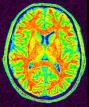
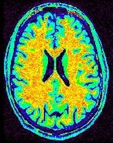
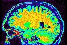
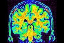
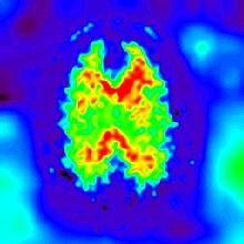
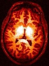
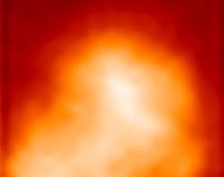
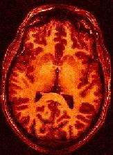
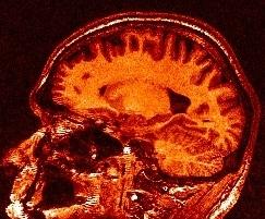
You may think that a unequivocal correspondence exists between the grey level in one voxel of a T1-weighted MR scan, and some esoteric property of the underlying cube of tissue. You should not succumb to this temptation. Take some time to observe a standard anatomical scan with a rainbow colormap to have this revelation:

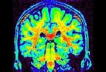
Some parts of the white matter are red, while some others are yellow or even green. All looks like as if the putative correspondence mentioned above was depending on the localization in the field of view. Usually, the center of the coil is lighter, but this is not a systematic observation and depends on the coil and scanner design. When one looks at a MR slice with a grey colormap, like in standard radiology, this default is not straightforward. Human vision, indeed, is very effective at correcting for this kind of spatial variations. This capacity has some link with the fact that we usually perceive object's colors as uniform, whatever illumination related variations. Unfortunately, this sophisticated feature of human vision has prevented the MR physicists to find the motivation to overcome that acquisition problem. Artificial vision still being in its infancy, it is much more disturbed by these spatial intensity variations than radiologists. This procedure has to correct for the spatial bias before any segmentation process can be reliably trigered.

The physical phenomena underlying the spatial inhomogeneities unfortunately depends on the shape of the subject's head. Hence, a systematic correction from an initial fantom based evaluation is not possible. A bias estimation has to be done for each new subject. Our approach to drive the estimation is to maximize a measure of the image quality after restoration. This measure is the entropy of the intensity distribution. A low entropy corresponds to an image where each tissue class is represented by a thin peak in the histogram. The spatial bias field leads to a thickening of the peaks, which increases the entropy.

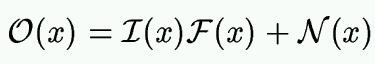
The simplest model standing for the origin of the observed intensities is the following:

The intensity observed in voxel x is supposed to correspond to the product between an intensity I intrinsic to the tissue and a spatial bias F, plus a RMN related noise. Some considerations about the multiple origins of the bias usually lead to assume spatial regularity. To restore image O, we estimate the bias F, assuming that the correcting field Fc has to maximize the measure of quality of the intrinsic image. Hence the optimal correction field minimizes the function:

The optimal field provides a trade-off between the quality measure (the entropy S(FcO)), the regularity of the field (R(Fc), a sum of quadratic discrepancies between neighbors), and a distance to the initial image (M(FcO), which discards the trivial solution corresponding to a constant intrinsic image). The K constants weight the influence of the three terms. The function is minimized first using simulated annealing at the highest level of a multigrid representation, where the field is piecewise constant. The field regularity is slightly relaxed when the grid resolution is increased. In our opinion, indeed, the ideal correcting field includes large variations at the level of T1 discontinuities. For the previous image, the resulting solution is the following:

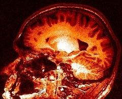
The intrinsic image:


The field F:


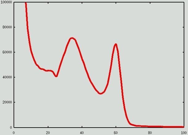
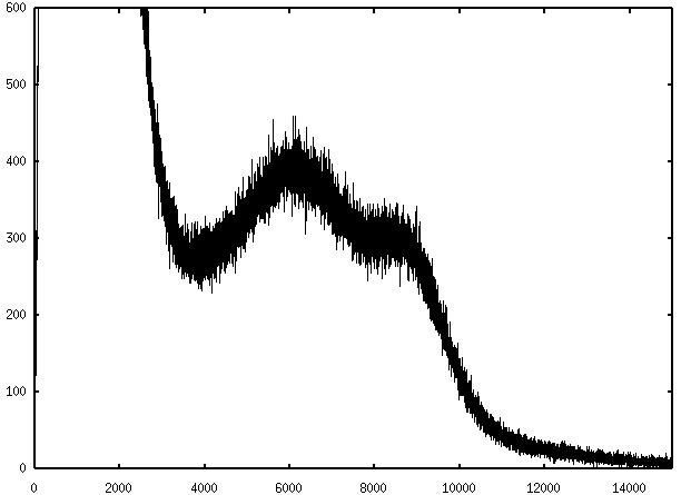
The histogram of the initial image O:


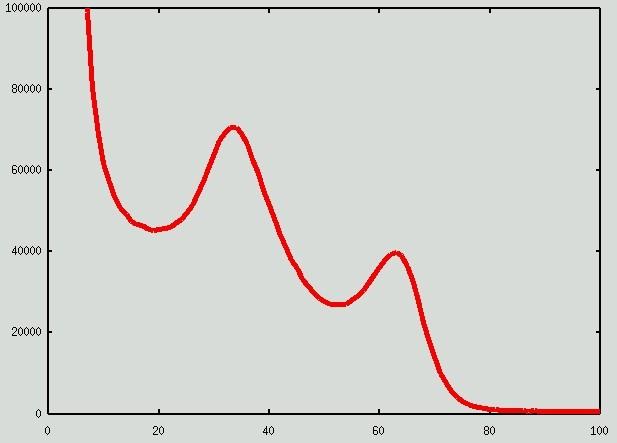
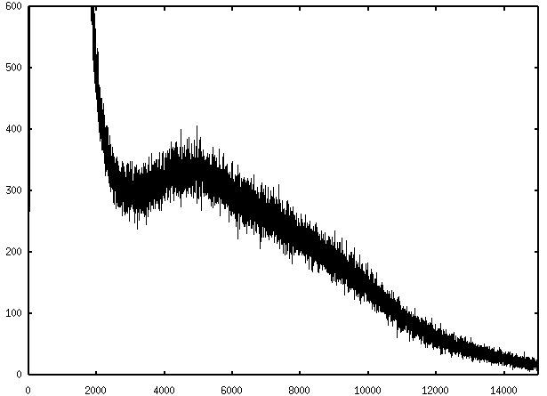
The histogram of the restored image I:


The main parameters to be tuned if you get some problems with your images are related to the field regularity:

• If the grey/white contrast of your images is weak, increase the field rigidity;
• If your coil leads to a high bias in the z direction (the magnet axes), lower the rigidity in that direction (zdir_multiply-regul between 0.1 and 1);
• If the intensities change from one slice to the neighboring ones, use the 2D mode (dim_rigidity).

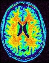
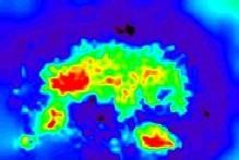
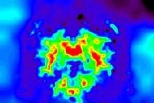
If your images stem from a high field magnet, the spatial bias may be especially high. In that case, you may have to lower the field rigidity. I guess you have understood now that a large bias with a low contrast may lead to some troubles... This procedure, however, can give correct results even when the grey and white peaks are completely mixed up:

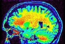
An example with our ten years old 3T magnet:


The estimated field:


The restored image:


For more information :
Entropy minimization for automatic correction of intensity non uniformity, J.-F. Mangin, MMBIA (Math. Methods in Biomed. Image Analysis), Hilton Head Island, South Carolina, IEEE Press 162-169, 2000

You can also try the commanline:
VipBiasCorrection -help

Parameters

mri: T1 MRI ( input )

any image (not necessarily T1-weighted)

mri_corrected: T1 MRI Bias Corrected ( output )

restored image

field_rigidity: Float ( input )

weight for the field rigidity constraint

write_field: Choice ( input )

dim_rigidity: Choice ( input )

2D leads to independent slices

sampling: Float ( input )

Block size, in mm, during simulated annealing

ngrid: Integer ( input )

Number of levels in the multigrid

geometric: Float ( input )

geometric decreasing of temperature

nIncrement: Choice ( input )

Transition number (*2) for the Gibbs sampler

init_temperature: Float ( input )

Initial temperature for annealing

increment: Float ( input )

init_amplitude: Float ( input )

zdir_multiply_regul: Float ( input )

Technical information

Toolbox : Morphologist

User level : 2

Identifier : VipBiasCorrection

File name : brainvisa/toolboxes/morphologist/processes/segmentationpipeline/components_obsolete/segmentation/VipBiasCorrection.py

Supported file formats :

mri :

gz compressed NIFTI-1 image, Aperio svs, BMP image, DICOM image, Directory, ECAT i image, ECAT v image, FDF image, FreesurferMGH, FreesurferMGZ, GIF image, GIS image, Hamamatsu ndpi, Hamamatsu vms, Hamamatsu vmu, JPEG image, Leica scn, MINC image, NIFTI-1 image, PBM image, PGM image, PNG image, PPM image, SPM image, Sakura svslide, TIFF image, TIFF image, TIFF(.tif) image, TIFF(.tif) image, VIDA image, Ventana bif, XBM image, XPM image, Zeiss czi, gz compressed MINC image, gz compressed NIFTI-1 image

mri_corrected :

gz compressed NIFTI-1 image, BMP image, DICOM image, Directory, ECAT i image, ECAT v image, FDF image, GIF image, GIS image, JPEG image, MINC image, NIFTI-1 image, PBM image, PGM image, PNG image, PPM image, SPM image, TIFF image, TIFF(.tif) image, VIDA image, XBM image, XPM image, gz compressed MINC image, gz compressed NIFTI-1 image