PyAims tutorial : programming with AIMS in Python language
This tutorial should work with Python 3 (Python 2 support has been dropped in pyaims 5.1).
This is a Jupyter/Ipython notebook:
pyaims_tutorial_nb.ipynb
AIMS is a C++ library, but has python language bindings: PyAIMS. This means that the C++ classes and functions can be used from python. This has many advantages compared to pure C++:
Writing python scripts and programs is much easier and faster than C++: there is no fastidious and long compilation step.
Scripts are more flexible, can be modified on-the-fly, etc
It can be used interactively in a python interactive shell.
As pyaims is actually C++ code called from python, it is still fast to execute complex algorithms. There is obviously an overhead to call C++ from python, but once in the C++ layer, it is C++ execution speed.
A few examples of how to use and manipulate the main data structures will be shown here.
The data for the examples in this section are available on the BrainVisa web site. New utility funcitons in pyaims 5.2 allow to download and install them very easily - see the beginning of the tutorial code. Alternatively they are here: https://brainvisa.info/download/data/test_data.zip.
[1]:
import sys
print(sys.version_info)
sys.version_info(major=3, minor=11, micro=0, releaselevel='final', serial=0)
[2]:
from soma.aims import demotools
import os
import tempfile

# let's work in a temporary directory
tuto_dir = tempfile.mkdtemp(prefix='pyaims_tutorial_')
older_cwd = os.getcwd()
# download/install demo data from the server, if not already done
demotools.install_demo_data('test_data.zip', install_dir=tuto_dir)

print('old cwd:', older_cwd)
os.chdir(tuto_dir)
print('we are working in:', tuto_dir)
download dir: /home_local/a-sac-ns-brainvisa/bbi-daily/brainvisa-web/build/share/brainvisa_demo
install dir: /tmp/pyaims_tutorial_8r066kp1
already downloaded, skipping download.
installing test_data.zip ...
old cwd: /home_local/a-sac-ns-brainvisa/bbi-daily/brainvisa-web/src/aims-free/pyaims/doc/sphinx
we are working in: /tmp/pyaims_tutorial_8r066kp1
We will need this function to print headers in a reproducible way in order to pass tests (it bascally removes the “referential” property which may be a randomly changing identifier).
[3]:
def clean_h(hdr, hidden=None):
    if hidden is None:
        hidden = set(['referential'])
    return {k: v for k, v in hdr.items() if k not in hidden}

def print_h(hdr, hidden=None):
    print(clean_h(hdr, hidden))
Using data structures
Module importation
In python, the aimsdata library is available as the soma.aims module.
[4]:
import soma.aims
# the module is actually soma.aims:
vol = soma.aims.Volume(100, 100, 100, dtype='int16')
or:
[5]:
from soma import aims
# the module is available as aims (not soma.aims):
vol = aims.Volume(100, 100, 100, dtype='int16')
# in the following, we will be using this form because it is shorter.
IO: reading and writing objects
Reading operations are accessed via a single soma.aims.read() function, and writing through a single soma.aims.write() function. soma.aims.read() function reads any object from a given file name, in any supported file format, and returns it:
[6]:
from soma import aims
obj = aims.read('data_for_anatomist/subject01/subject01.nii')
print(obj.getSize())
obj2 = aims.read('data_for_anatomist/subject01/Audio-Video_T_map.nii')
print(obj2.getSize())
obj3 = aims.read('data_for_anatomist/subject01/subject01_Lhemi.mesh')
print(len(obj3.vertex(0)))
assert(obj.getSize() == [256, 256, 124, 1])
assert(obj2.getSize() == [53, 63, 46, 1])
assert(obj3.size() == 1 and len(obj3.vertex(0)) == 33837)
[256, 256, 124, 1]
[53, 63, 46, 1]
33837
The returned object can have various types according to what is found in the disk file(s).
Writing is just as easy. The file name extension generally determines the output format. An object read from a given format can be re-written in any other supported format, provided the format can actually store the object type.
[7]:
from soma import aims
obj2 = aims.read('data_for_anatomist/subject01/Audio-Video_T_map.nii')
aims.write(obj2, 'Audio-Video_T_map.ima')
obj3 = aims.read('data_for_anatomist/subject01/subject01_Lhemi.mesh')
aims.write(obj3, 'subject01_Lhemi.gii')
Exercise
Write a little file format conversion tool
Volumes
Volumes are array-like containers of voxels, plus a set of additional information kept in a header structure. In AIMS, the header structure is generic and extensible, and does not depend on a specific file format. Voxels may have various types, so a specific type of volume should be used for a specific type of voxel. The type of voxel has a code that is used to suffix the Volume type: soma.aims.Volume_S16 for signed 16-bit ints, soma.aims.Volume_U32 for unsigned 32-bit ints, soma.aims.Volume_FLOAT for 32-bit floats, soma.aims.Volume_DOUBLE for 64-bit floats, soma.aims.Volume_RGBA for RGBA colors, etc.
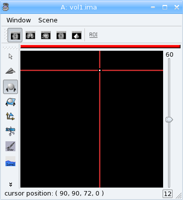
Building a volume
[8]:
 # create a 3D volume of signed 16-bit ints, of size 192x256x128
vol = aims.Volume(192, 256, 128, dtype='int16')
# fill it with zeros
vol.fill(0)
# set value 12 at voxel (100, 100, 60)
vol.setValue(12, 100, 100, 60)
# get value at the same position
x = vol.value(100, 100, 60)
print(x)
assert(x == 12)
12
[9]:
# using the array accessors
vol[100, 100, 60, 0] = 0
print(vol.value(100, 100, 60))
vol[100, 100, 60, 0] = 12
print(vol[100, 100, 60, 0])
0
12
[10]:
# set the voxels size
vol.header()['voxel_size'] = [0.9, 0.9, 1.2, 1.]
print(vol.header())
assert(clean_h(vol.header()) ==
       {'sizeX': 192, 'sizeY': 256, 'sizeZ': 128, 'sizeT': 1, 'voxel_size': [0.9, 0.9, 1.2, 1],
        'volume_dimension': [192, 256, 128, 1]})
{ 'volume_dimension' : [ 192, 256, 128, 1 ], 'sizeX' : 192, 'sizeY' : 256, 'sizeZ' : 128, 'sizeT' : 1, 'referential' : 'dcf64580-7634-11f1-9e12-8c8474907e8e', 'voxel_size' : [ 0.9, 0.9, 1.2, 1 ] }
Basic operations
Whole volume operations:
[11]:
# multiplication, addition etc
vol *= 2
vol2 = vol * 3 + 12
print(vol2.value(100, 100, 60))
vol /= 2
vol3 = vol2 - vol - 12
print(vol3.value(100, 100, 60))
vol4 = vol2 * vol / 6
print(vol4.value(100, 100, 60))
assert(vol2.value(100, 100, 60) == 84)
assert(vol3.value(100, 100, 60) == 60)
assert(vol4.value(100, 100, 60) == 168)
84
60
168
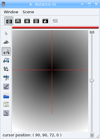
Voxel-wise operations:
[12]:
# fill the volume with the distance to voxel (100, 100, 60)
vs = vol.header()['voxel_size']
pos0 = (100 * vs[0], 100 * vs[1], 60 * vs[2]) # in millimeters
for z in range(vol.getSizeZ()):
    for y in range(vol.getSizeY()):
        for x in range(vol.getSizeX()):
            # get current position in an aims.Point3df structure, in mm
            p = aims.Point3df(x * vs[0], y * vs[1], z * vs[2])
            # get relative position to pos0, in voxels
            p -= pos0
            # distance: norm of vector p
            dist = int(round(p.norm()))
            # set it into the volume
            vol.setValue(dist, x, y, z)
print(vol.value(100, 100, 60))
# save the volume
aims.write(vol, 'distance.nii')
assert(vol.value(100, 100, 60) == 0)
0
Now look at the distance.nii volume in Anatomist.
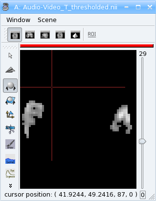
Exercise
Make a program which loads the image data_for_anatomist/subject01/Audio-Video_T_map.nii and thresholds it so as to keep values above 3.
[13]:
from soma import aims
vol = aims.read('data_for_anatomist/subject01/Audio-Video_T_map.nii')
print(vol.value(20, 20, 20) < 3. and vol.value(20, 20, 20) != 0.)
assert(vol.value(20, 20, 20) < 3. and vol.value(20, 20, 20) != 0.)
for z in range(vol.getSizeZ()):
    for y in range(vol.getSizeY()):
        for x in range(vol.getSizeX()):
            if vol.value(x, y, z) < 3.:
                vol.setValue(0, x, y, z)
print(vol.value(20, 20, 20))
aims.write(vol, 'Audio-Video_T_thresholded.nii')
assert(vol.value(20, 20, 20) == 0.)
True
0.0
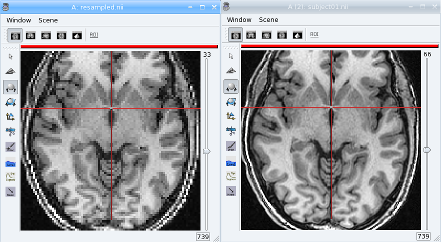
Exercise
Make a program to dowsample the anatomical image data_for_anatomist/subject01/subject01.nii and keeps one voxel out of two in every direction.
[14]:
from soma import aims
vol = aims.read('data_for_anatomist/subject01/subject01.nii')
# allocate a new volume with half dimensions
vol2 = aims.Volume(vol.getSizeX() // 2, vol.getSizeY() // 2, vol.getSizeZ() // 2, dtype='DOUBLE')
print(vol2.getSizeX())
assert(vol2.getSizeX() == 128)
# set the voxel size to twice it was in vol
vs = vol.header()['voxel_size']
vs2 = [x * 2 for x in vs]
vol2.header()['voxel_size'] = vs2
for z in range(vol2.getSizeZ()):
    for y in range(vol2.getSizeY()):
        for x in range(vol2.getSizeX()):
            vol2.setValue(vol.value(x*2, y*2, z*2), x, y, z)
print(vol.value(100, 100, 40))
print(vol2.value(50, 50, 20))
aims.write(vol2, 'resampled.nii')
assert(vol.value(100, 100, 40) == 775)
assert(vol2.value(50, 50, 20) == 775.)
128
775
775.0
The first thing that comes to mind when running these examples, is that they are slow. Indeed, python is an interpreted language and loops in any interpreted language are slow. In addition, accessing individually each voxel of the volume has the overhead of python/C++ bindings communications. The conclusion is that that kind of example is probably a bit too low-level, and should be done, when possible, by compiled libraries or specialized array-handling libraries. This is the role of numpy.
Accessing numpy arrays to AIMS volume voxels is supported:
[15]:
import numpy
vol.fill(0)
arr = numpy.asarray(vol)
# or:
arr = vol.np
# set value 100 in a whole sub-volume
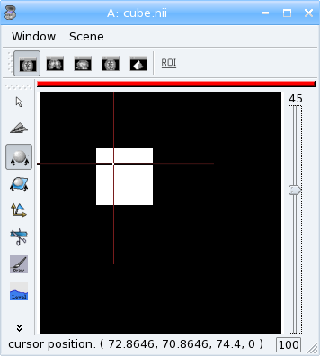
arr[60:120, 60:120, 40:80] = 100
# note that arr is a shared view to the volume contents,
# modifications will also affect the volume
print(vol.value(65, 65, 42))
print(vol.value(65, 65, 30))
aims.write(vol, "cube.nii")
assert(vol.value(65, 65, 42) == 100)
assert(vol.value(65, 65, 30) == 0)
100
0
We can also use numpy accessors and slicing features directly on a Volume object:
[16]:
vol.fill(0)
vol[60:120, 60:120, 40:80] = 100
print(vol.value(65, 65, 42))
print(vol.value(65, 65, 30))
assert(numpy.all(vol[65, 65, 42, 0] == 100))
assert(numpy.all(vol[65, 65, 30, 0] == 0))
100
0
Now we can re-write the thresholding example using numpy:
[17]:
from soma import aims
vol = aims.read('data_for_anatomist/subject01/Audio-Video_T_map.nii')
arr = vol.np
arr[arr < 3.] = 0.
print(vol[20, 20, 20, 0])
aims.write(vol, 'Audio-Video_T_thresholded2.nii')
assert(vol[20, 20, 20, 0] == 0)
0.0
Here, arr < 3. returns a boolean array with the same size as arr. We can even use shortcuts on the Volume object:
[18]:
from soma import aims
vol = aims.read('data_for_anatomist/subject01/Audio-Video_T_map.nii')
vol[vol.np < 3.] = 0.
print(vol[20, 20, 20, 0])
aims.write(vol, 'Audio-Video_T_thresholded3.nii')
assert(vol[20, 20, 20, 0] == 0)
0.0
The distance example, using numpy, would like the following:
[19]:
from soma import aims
import numpy
vol = aims.Volume(192, 256, 128, 'S16')
vol.header()['voxel_size'] = [0.9, 0.9, 1.2, 1.]
vs = vol.header()['voxel_size']
pos0 = (100 * vs[0], 100 * vs[1], 60 * vs[2]) # in millimeters
# build arrays of coordinates for x, y, z
x, y, z = numpy.ogrid[0.:vol.getSizeX(), 0.:vol.getSizeY(), 0.:vol.getSizeZ()]
# get coords in millimeters
x *= vs[0]
y *= vs[1]
z *= vs[2]
# relative to pos0
x -= pos0[0]
y -= pos0[1]
z -= pos0[2]
# get norm, using numpy arrays broadcasting
vol[:, :, :, 0] = numpy.sqrt(x**2 + y**2 + z**2)

print(vol[100, 100, 60, 0])
assert(vol[100, 100, 60, 0] == 0)

# and save result
aims.write(vol, 'distance2.nii')
0
This example appears a bit more tricky, since we must build the coordinates arrays, but is way faster to execute, because all loops within the code are executed in compiled routines in numpy. One interesting thing to note is that this code is using the famous “array broadcasting” feature of numpy, where arrays of heterogeneous sizes can be combined, and the “missing” dimensions are extended.
Copying volumes or volumes structure, or building from an array
To make a deep-copy of a volume, use the copy constructor:
[20]:
vol2 = aims.Volume(vol)
vol2[100, 100, 60, 0] = 12
# now vol and vol2 have different values
print('vol.value(100, 100, 60):', vol.value(100, 100, 60))
assert(vol.value(100, 100, 60) == 0)
print('vol2.value(100, 100, 60):', vol2.value(100, 100, 60))
assert(vol2.value(100, 100, 60) == 12)
vol.value(100, 100, 60): 0
vol2.value(100, 100, 60): 12
If you need to build another, different volume, with the same structure and size, don’t forget to copy the header part:
[21]:
vol2 = aims.Volume(vol.getSize(), 'FLOAT')
vol2.copyHeaderFrom(vol.header())
print(vol2.header())
assert(clean_h(vol2.header())
       == {'sizeX': 192, 'sizeY': 256, 'sizeZ': 128, 'sizeT': 1, 'voxel_size': [0.9, 0.9, 1.2, 1],
           'volume_dimension': [192, 256, 128, 1]})
{ 'volume_dimension' : [ 192, 256, 128, 1 ], 'sizeX' : 192, 'sizeY' : 256, 'sizeZ' : 128, 'sizeT' : 1, 'referential' : 'ec04bcd2-7634-11f1-9e12-8c8474907e8e', 'voxel_size' : [ 0.9, 0.9, 1.2, 1 ] }
Important information can reside in the header, like voxel size, or coordinates systems and geometric transformations to other coordinates systems, so it is really very important to carry this information with duplicated or derived volumes.
You can also build a volume from a numpy array:
[22]:
arr = numpy.array(numpy.diag(range(40)), dtype=numpy.float32).reshape(40, 40, 1) \
    + numpy.array(range(20), dtype=numpy.float32).reshape(1, 1, 20)
# WARNING: AIMS used to require an array in Fortran ordering,
# whereas the numpy addition always returns a C-ordered array
# in 5.1 this limitation is gone, hwever many C++ algorithms will not work
# (and probably crash) with a C-aligned numpy array. If you need, ask a
# fortran orientation this way:
# arr = numpy.array(arr, order='F')
# for today, let's use the C ordered array:
arr[10, 12, 3] = 25
vol = aims.Volume(arr)
print('vol.value(10, 12, 3):', vol.value(10, 12, 3))
assert(vol.value(10, 12, 3) == 25.)

# data are shared with arr
vol.setValue(35, 10, 15, 2)
print('arr[10, 15, 2]:', arr[10, 15, 2])
assert(arr[10, 15, 2] == 35.0)
arr[12, 15, 1] = 44
print('vol.value(12, 15, 1):', vol.value(12, 15, 1))
assert(vol.value(12, 15, 1) == 44.0)
vol.value(10, 12, 3): 25.0
arr[10, 15, 2]: 35.0
vol.value(12, 15, 1): 44.0
4D volumes
4D volumes work just like 3D volumes. Actually all volumes are 4D in AIMS, but the last dimension is commonly of size 1. In soma.aims.Volume_FLOAT.value and soma.aims.Volume_FLOAT.setValue methods, only the first dimension is mandatory, others are optional and default to 0, but up to 4 coordinates may be used. In the same way, the constructor takes up to 4 dimension parameters:
[23]:
from soma import aims
# create a 4D volume of signed 16-bit ints, of size 30x30x30x4
vol = aims.Volume(30, 30, 30, 4, 'S16')
# fill it with zeros
vol.fill(0)
# set value 12 at voxel (10, 10, 20, 2)
vol.setValue(12, 10, 10, 20, 2)
# get value at the same position
x = vol.value(10, 10, 20, 2)
print(x)
assert(x == 12)
# set the voxels size
vol.header()['voxel_size'] = [0.9, 0.9, 1.2, 1.]
print(vol.header())
assert(clean_h(vol.header())
       == {'sizeX': 30, 'sizeY': 30, 'sizeZ': 30, 'sizeT': 4, 'voxel_size': [0.9, 0.9, 1.2, 1],
           'volume_dimension': [30, 30, 30, 4]})
12
{ 'volume_dimension' : [ 30, 30, 30, 4 ], 'sizeX' : 30, 'sizeY' : 30, 'sizeZ' : 30, 'sizeT' : 4, 'referential' : 'ec280322-7634-11f1-9e12-8c8474907e8e', 'voxel_size' : [ 0.9, 0.9, 1.2, 1 ] }
Similarly, 1D or 2D volumes may be used exactly the same way.
Volume views and subvolumes
A volume can be a view into another volume. This is a way of handling “border” with Volume:
[24]:
vol = aims.Volume(14, 14, 14, 1, dtype='int16')
print('large volume size:', vol.shape)
vol.fill(0)
# take a view at position (2, 2, 2, 0) and size (10, 10, 10, 1)
view = aims.VolumeView(vol, [2, 2, 2, 0], [10, 10, 10, 1])
print('view size:', view.shape)
assert(view.posInRefVolume() == (2, 2, 2, 0) and view.shape == (10, 10, 10, 1))
view[0, 0, 0, 0] = 45
assert(vol[2, 2, 2, 0] == 45)
# view is actually a regular Volume
print(type(view))
large volume size: (14, 14, 14, 1)
view size: (10, 10, 10, 1)
<class 'soma.aims.Volume_S16'>
Partial IO
Some volume IO formats implemented in the Soma-IO library support partial IO and reading a view inside a larger volume (since pyaims 5.1). Be careful, all formats do not support these operations.
[25]:
# get volume dimension on file
import os
os.chdir(tuto_dir)
f = aims.Finder()
f.check('data_for_anatomist/subject01/subject01.nii')
# allocate a large volume
vol = aims.Volume(300, 300, 200, 1, dtype=f.dataType())
vol.fill(0)
view = aims.VolumeView(vol, [20, 20, 20, 0], f.header()['volume_dimension'])
print('view size:', view.shape)
# read the view. the otion "keep_allocation" is important
# in order to prevent re-allocation of the volume.
aims.read('data_for_anatomist/subject01/subject01.nii', object=view, options={'keep_allocation': True})
print(view[100, 100, 64, 0])
assert(view[100, 100, 64, 0] == vol[120, 120, 84, 0])
# otherwise we can read part of a volume
view2 = aims.VolumeView(vol, (100, 100, 40, 0), (50, 50, 50, 1))
aims.read('data_for_anatomist/subject01/subject01.nii', object=view2,
          options={'keep_allocation': True, 'ox': 60, 'sx': 50,
                   'oy': 50, 'sy': 50, 'sz': 50})
print(view2[20, 20, 20, 0], vol[120, 120, 60, 0], view[100, 100, 40, 0])
print(view2.shape, view.shape, vol.shape)
assert(view2[20, 20, 20, 0] == vol[120, 120, 60, 0])
assert(view2[20, 20, 20, 0] == view[100, 100, 40, 0])
# view2 is shifted compared to view, check it
assert(view2[20, 20, 20, 0] == view[80, 70, 20, 0])
view size: (256, 256, 124, 1)
667
94 94 94
(50, 50, 50, 1) (256, 256, 124, 1) (300, 300, 200, 1)
Meshes
Structure
A surfacic mesh represents a surface, as a set of small polygons (generally triangles, but sometimes quads). It has two main components: a vector of vertices (each vertex is a 3D point, with coordinates in millimeters), and a vector of polygons: each polygon is defined by the vertices it links (3 for a triangle). It also optionally has normals (unit vectors). In our mesh structures, there is one normal for each vertex.
[26]:
from soma import aims
mesh = aims.read('data_for_anatomist/subject01/subject01_Lhemi.mesh')
vert = mesh.vertex()
print('vertices:', len(vert))
assert(len(vert) == 33837)
poly = mesh.polygon()
print('polygons:', len(poly))
assert(len(poly) == 67678)
norm = mesh.normal()
print('normals:', len(norm))
assert(len(norm) == 33837)
vertices: 33837
polygons: 67678
normals: 33837
To build a mesh, we can instantiate an object of type aims.AimsTimeSurface_<n>_VOID, for example soma.aims.AimsTimeSurface_3_VOID, with n being the number of vertices by polygon. VOID means that the mesh has no texture in it (which we generally don’t use, we prefer using texture as separate objects). Then we can add vertices, normals and polygons to the mesh:
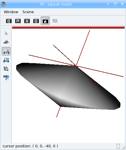
[27]:
# build a flying saucer mesh
from soma import aims
import numpy
mesh = aims.AimsTimeSurface(3)
# a mesh has a header
mesh.header()['toto'] = 'a message in the header'
vert = mesh.vertex()
poly = mesh.polygon()
x = numpy.cos(numpy.ogrid[0.: 20] * numpy.pi / 10.) * 100
y = numpy.sin(numpy.ogrid[0.: 20] * numpy.pi / 10.) * 100
z = numpy.zeros(20)
c = numpy.vstack((x, y, z)).transpose()
vert.assign(numpy.vstack((numpy.array([(0., 0., -40.), (0., 0., 40.)]), c)))
pol = numpy.vstack((numpy.zeros(20, dtype=numpy.int32), numpy.ogrid[3: 23], numpy.ogrid[2: 22])).transpose()
pol[19, 1] = 2
pol2 = numpy.vstack((numpy.ogrid[2: 22], numpy.ogrid[3: 23], numpy.ones(20, dtype=numpy.int32))).transpose()
pol2[19, 1] = 2
poly.assign(numpy.vstack((pol, pol2)))
# write result
aims.write(mesh, 'saucer.gii')
# automatically calculate normals
mesh.updateNormals()
Modifying a mesh
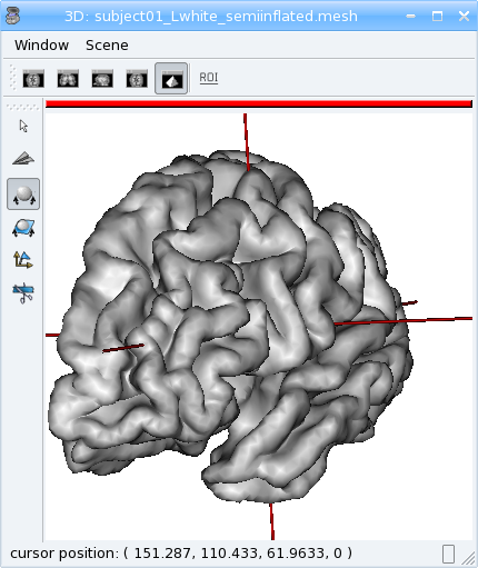
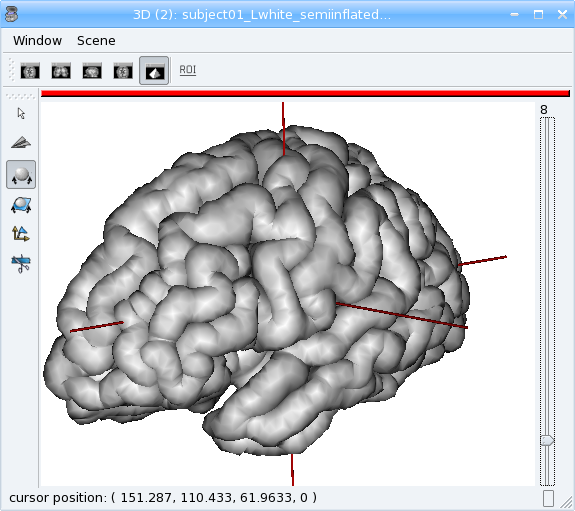
[28]:
# slightly inflate a mesh
from soma import aims
import numpy
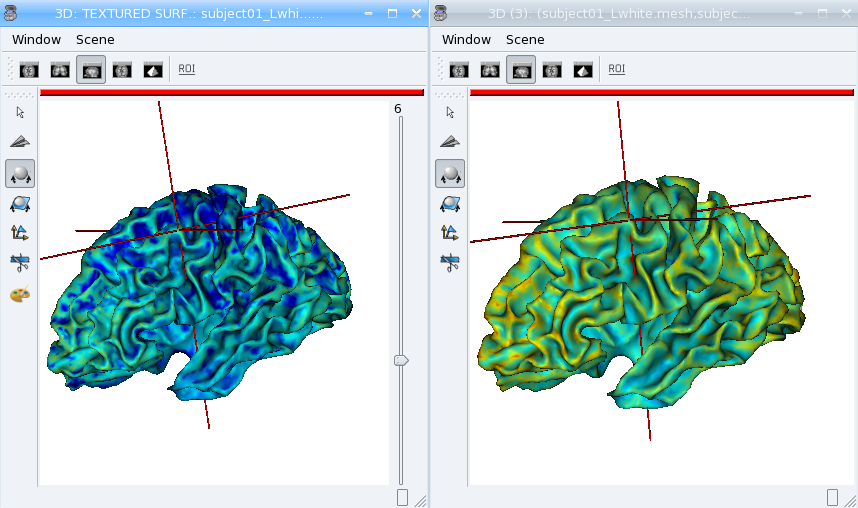
mesh = aims.read('data_for_anatomist/subject01/subject01_Lwhite.mesh')
vert = numpy.asarray(mesh.vertex())
norm = numpy.asarray(mesh.normal())
vert += norm * 2 # push vertices 2mm away along normal
mesh.updateNormals()
aims.write(mesh, 'subject01_Lwhite_semiinflated.mesh')
Now look at both meshes in Anatomist…
Note that this code only works this way from pyaims 4.7, earlier versions had to reassign the coordinates array to the vertices vector of the mesh.
Alternatively, without numpy, we could have written the code like this:
[29]:
mesh = aims.read('data_for_anatomist/subject01/subject01_Lwhite.mesh')
vert = mesh.vertex()
norm = mesh.normal()
for v, n in zip(vert, norm):
    v += n * 2
mesh.updateNormals()
aims.write(mesh, 'subject01_Lwhite_semiinflated.mesh')
Handling time
In AIMS, meshes are actually time-indexed dictionaries of meshes. This way a deforming mesh can be stored in the same object. To copy a timestep to another, use the following:
[30]:
from soma import aims
mesh = aims.read('data_for_anatomist/subject01/subject01_Lwhite.mesh')
# mesh.vertex() is equivalent to mesh.vertex(0)
mesh.vertex(1).assign(mesh.vertex(0))
# same for normals and polygons
mesh.normal(1).assign(mesh.normal(0))
mesh.polygon(1).assign(mesh.polygon(0))
print('number of time steps:', mesh.size())
assert(mesh.size() == 2)
number of time steps: 2
Exercise
Make a deforming mesh that goes from the original mesh to 5mm away, by steps of 0.5 mm
[31]:
from soma import aims
import numpy
mesh = aims.read('data_for_anatomist/subject01/subject01_Lwhite.mesh')
vert = numpy.array(mesh.vertex())  # must make an actual copy to avoid modifying timestep 0
norm = numpy.asarray(mesh.normal())
for i in range(1, 10):
    mesh.polygon(i).assign(mesh.polygon())
    vert += norm * 0.5
    mesh.vertex(i).assign(vert)
    # don't bother about normals, we will rebuild them afterwards.
print('number of time steps:', mesh.size())
assert(mesh.size() == 10)
mesh.updateNormals()  # I told you about normals.
aims.write(mesh, 'subject01_Lwhite_semiinflated_time.mesh')
number of time steps: 10
Textures
A texture is merely a vector of values, each of them is assigned to a mesh vertex, with a one-to-one mapping, in the same order. A texture is also a time-texture.
[32]:
from soma import aims
tex = aims.TimeTexture('FLOAT')
t = tex[0] # time index, inserts on-the-fly
t.reserve(10) # pre-allocates memory
for i in range(10):
    t.append(i / 10.)
print(tex.size())
assert(len(tex) == 1)
print(tex[0].size())
assert(len(tex[0]) == 10)
print(tex[0][5])
assert(tex[0][5] == 0.5)
1
10
0.5
Exercise
Make a time-texture, with at each time/vertex of the previous mesh, sets the value of the underlying volume data_for_anatomist/subject01/subject01.nii
[33]:
from soma import aims
import numpy as np

mesh = aims.read('subject01_Lwhite_semiinflated_time.mesh')
vol = aims.read('data_for_anatomist/subject01/subject01.nii')
tex = aims.TimeTexture('FLOAT')
vs = vol.header()['voxel_size']
for i in range(mesh.size()):
    vert = np.asarray(mesh.vertex(i))
    tex[i].assign(np.zeros((len(vert),), dtype=np.float32))
    t = np.asarray(tex[i])
    coords = np.zeros((len(vert), len(vol.shape)), dtype=int)
    coords[:, :3] = np.round(vert / vs).astype(int)
    t[:] = vol[tuple(coords.T)]
aims.write(tex, 'subject01_Lwhite_semiinflated_texture.tex')
Now look at the texture on the mesh (inflated or not) in Anatomist. Compare it to a 3D fusion between the mesh and the MRI volume.
Bonus: We can do the same for functional data. But in this case we may have a spatial transformation to apply between anatomical data and functional data (which may have been normalized, or acquired in a different referential).
[34]:
from soma import aims
import numpy as np
mesh = aims.read('subject01_Lwhite_semiinflated_time.mesh')
vol = aims.read('data_for_anatomist/subject01/Audio-Video_T_map.nii')
# get header info from anatomical volume
f = aims.Finder()
assert(f.check('data_for_anatomist/subject01/subject01.nii'))
anathdr = f.header()
# get functional -> MNI transformation
m1 = aims.AffineTransformation3d(vol.header()['transformations'][1])
# get anat -> MNI transformation
m2 = aims.AffineTransformation3d(anathdr['transformations'][1])
# make anat -> functional transformation
anat2func = m1.inverse() * m2
# include functional voxel size to get to voxel coordinates
vs = vol.header()['voxel_size']
mvs = aims.AffineTransformation3d(np.diag(vs[:3] + [1.]))
anat2func = mvs.inverse() * anat2func
# now go as in the previous program
tex = aims.TimeTexture('FLOAT')
for i in range(mesh.size()):
    vert = np.asarray(mesh.vertex(i))
    tex[i].assign(np.zeros((len(vert),), dtype=np.float32))
    t = np.asarray(tex[i])
    coords = np.ones((len(vert), len(vol.shape)), dtype=np.float32)
    coords[:, :3] = vert
    # apply matrix anat2func to coordinates array
    coords = np.round(coords.dot(anat2func.toMatrix().T)).astype(int)
    coords[:, 3] = 0
    t[:] = vol[tuple(coords.T)]
aims.write(tex, 'subject01_Lwhite_semiinflated_audio_video.tex')
See how the functional data on the mesh changes across the depth of the cortex. This demonstrates the need to have a proper projection of functional data before dealing with surfacic functional processing.
Buckets
“Buckets” are voxels lists. They are typically used to represent ROIs. A BucketMap is a list of Buckets. Each Bucket contains a list of voxels coordinates. A BucketMap is represented by the class soma.aims.BucketMap_VOID.
[35]:
from soma import aims
bck_map=aims.read('data_for_anatomist/roi/basal_ganglia.data/roi_Bucket.bck')
print('Bucket map: ', bck_map)
print('Nb buckets: ', bck_map.size())
assert(bck_map.size() == 15)
for i in range(bck_map.size()):
    b = bck_map[i]
    print("Bucket", i, ", nb voxels:", b.size())
    if b.keys():
        print("  Coordinates of the first voxel:", b.keys()[0].list())
assert(bck_map[0].size() == 2314)
assert(bck_map[0].keys()[0] == [108, 132, 44])
Bucket map:  <soma.aims.BucketMap_VOID object at 0x7b5857b889d0>
Nb buckets:  15
Bucket 0 , nb voxels: 2314
  Coordinates of the first voxel: [108, 132, 44]
Bucket 1 , nb voxels: 2119
  Coordinates of the first voxel: [108, 108, 53]
Bucket 2 , nb voxels: 2639
  Coordinates of the first voxel: [100, 122, 52]
Bucket 3 , nb voxels: 1444
  Coordinates of the first voxel: [107, 128, 57]
Bucket 4 , nb voxels: 715
  Coordinates of the first voxel: [107, 112, 67]
Bucket 5 , nb voxels: 2171
  Coordinates of the first voxel: [143, 130, 44]
Bucket 6 , nb voxels: 2154
  Coordinates of the first voxel: [142, 111, 53]
Bucket 7 , nb voxels: 2063
  Coordinates of the first voxel: [149, 128, 52]
Bucket 8 , nb voxels: 1588
  Coordinates of the first voxel: [140, 130, 57]
Bucket 9 , nb voxels: 1012
  Coordinates of the first voxel: [144, 114, 67]
Bucket 10 , nb voxels: 8240
  Coordinates of the first voxel: [114, 136, 44]
Bucket 11 , nb voxels: 2159
  Coordinates of the first voxel: [97, 130, 52]
Bucket 12 , nb voxels: 2931
  Coordinates of the first voxel: [149, 130, 52]
Bucket 13 , nb voxels: 6279
  Coordinates of the first voxel: [112, 145, 50]
Bucket 14 , nb voxels: 6502
  Coordinates of the first voxel: [133, 147, 50]
Graphs
Graphs are data structures that may contain various elements. They can represent sets of smaller structures, and also relations between such structures. The main usage we have for them is to represent ROIs sets, sulci, or fiber bundles. A graph is represented by the class soma.aims.Graph.
A graph contains:
properties of any type, like a volume or mesh header.
nodes (also called vertices), which represent structured elements (a ROI, a sulcus part, etc), which in turn can store properties, and geometrical elements: buckets, meshes…
optionally, relations, which link nodes and can also contain properties and geometrical elements.
Properties
Properties are stored in a dictionary-like way. They can hold almost anything, but a restricted set of types can be saved and loaded. It is exactly the same thing as headers found in volumes, meshes, textures or buckets.
[36]:
from soma import aims
graph = aims.read('data_for_anatomist/roi/basal_ganglia.arg')
print(graph)
assert(repr(graph).startswith("{ '__syntax__' : 'RoiArg', 'RoiArg_VERSION' : '1.0', "
                              "'filename_base' : 'basal_ganglia.data',"))
print('properties:', graph.keys())
assert(len([x in graph.keys()
            for x in ('RoiArg_VERSION', 'filename_base', 'roi.global.bck',
                      'type.global.bck', 'boundingbox_max')]) == 5)
for p, v in graph.items():
    print(p, ':', v)
graph['gudule'] = [12, 'a comment']
{ '__syntax__' : 'RoiArg', 'RoiArg_VERSION' : '1.0', 'filename_base' : 'basal_ganglia.data', 'roi.global.bck' : 'roi roi_Bucket.bck roi_label', 'type.global.bck' : 'roi.global.bck', 'boundingbox_max' : [ 255, 255, 123 ], 'boundingbox_min' : [ 0, 0, 0 ], 'voxel_size' : [ 0.9375, 0.9375, 1.20000004768372 ], 'object_attributes_colors' : <Can't write data of type rc_ptr of map of string_vector of S32 in >, 'aims_objects_table' : <Can't write data of type rc_ptr of map of string_map of string_GraphElementCode in >, 'aims_reader_filename' : 'data_for_anatomist/roi/basal_ganglia.arg', 'aims_reader_loaded_objects' : 3, 'header' : { 'arg_syntax' : 'RoiArg', 'data_type' : 'VOID', 'file_type' : 'ARG', 'object_type' : 'Graph' } }
properties: ('RoiArg_VERSION', 'filename_base', 'roi.global.bck', 'type.global.bck', 'boundingbox_max', 'boundingbox_min', 'voxel_size', 'object_attributes_colors', 'aims_objects_table', 'aims_reader_filename', 'aims_reader_loaded_objects', 'header')
RoiArg_VERSION : 1.0
filename_base : basal_ganglia.data
roi.global.bck : roi roi_Bucket.bck roi_label
type.global.bck : roi.global.bck
boundingbox_max : [255, 255, 123]
boundingbox_min : [0, 0, 0]
voxel_size : [0.9375, 0.9375, 1.2]
object_attributes_colors : <Can't write data of type rc_ptr of map of string_vector of S32 in >
aims_objects_table : <Can't write data of type rc_ptr of map of string_map of string_GraphElementCode in >
aims_reader_filename : data_for_anatomist/roi/basal_ganglia.arg
aims_reader_loaded_objects : 3
header : { 'arg_syntax' : 'RoiArg', 'data_type' : 'VOID', 'file_type' : 'ARG', 'object_type' : 'Graph' }
Warning: wrong filename_base in graph, trying to fix it
Note
Only properties declared in a “syntax” file may be saved and re-loaded. Other properties are just not saved.
Vertices
Vertices (or nodes) can be accessed via the vertices() method. Each vertex is also a dictionary-like properties set.
[37]:
for v_name in sorted([v['name'] for v in graph.vertices()]):
    print(v_name)
Caude_droit
Caude_gauche
Corps_caude_droit
Corps_caude_gauche
Pallidum_droit
Pallidum_gauche
Putamen_droit_ant
Putamen_droit_post
Putamen_gauche_ant
Putamen_gauche_post
Striatum_ventral_droit
Striatum_ventral_gauche
Thalamus_droit
Thalamus_gauche
v1v2v3
To insert a new vertex, the soma.aims.Graph.addVertex() method should be used:
[38]:
v = graph.addVertex('roi')
print(v)
assert(v.getSyntax() == 'roi')
v['name'] = 'new ROI'
print(v)
assert(v == {'name': 'new ROI'})
{ '__syntax__' : 'roi' }
{ '__syntax__' : 'roi', 'name' : 'new ROI' }
Edges
An edge, or relation, links nodes together. Up to now we have always used binary, unoriented, edges. They can be added using the soma.aims.Graph.addEdge() method. Edges are also dictionary-like properties sets.
[39]:
v2 = [x for x in graph.vertices() if x['name'] == 'Pallidum_gauche'][0]
e = graph.addEdge(v, v2, 'roi_link')
print(graph.edges())
# get vertices linked by this edge
print(sorted([x['name'] for x in e.vertices()]))
assert(sorted([x['name'] for x in e.vertices()]) == ['Pallidum_gauche', 'new ROI'])
[ { '__syntax__' : 'roi_link' } ]
['Pallidum_gauche', 'new ROI']
### Adding meshes or buckets in a graph vertex or relation
Setting meshes or buckets in vertices properties is OK internally, but for saving and loading, additional consistancy must be ensured and internal tables update is required. Then, use the soma.aims.GraphManip.storeAims function:
[40]:
mesh = aims.read('data_for_anatomist/subject01/subject01_Lwhite.mesh')
# store mesh in the 'roi' property of vertex v of graph graph
aims.GraphManip.storeAims(graph, v, 'roi', mesh)
Other examples
There are other examples for pyaims here.
Using algorithms
AIMS contains, in addition to the different data structures used in neuroimaging, a set of algorithms which operate on these structures. Currently only a few of them have Python bindings, because we develop these bindings in a “lazy” way, only when they are needed. The algorithms currently available include data conversion, resampling, thresholding, mathematical morphology, distance maps, the mesher, some mesh generators, and a few others. But most of the algorithms are still only available in C++.
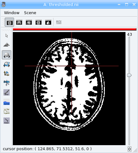
Volume Thresholding
[41]:
from soma import aims, aimsalgo
# read a volume with 2 voxels border
vol = aims.read('data_for_anatomist/subject01/subject01.nii', border=2)
# use a thresholder which will keep values above 600
ta = aims.AimsThreshold(aims.AIMS_GREATER_OR_EQUAL_TO, 600, intype=vol)
print('vol:', vol.getSize())
# use it to make a binary thresholded volume
tvol = ta.bin(vol)
print(tvol.value(0, 0, 0))
assert(tvol.value(0, 0, 0) == 0)
print(tvol.value(100, 100, 50))
assert(tvol.value(100, 100, 50) == 32767)
aims.write(tvol, 'thresholded.nii')
vol: [256, 256, 124, 1]
0
32767
Warning
warning:: Some algorithms need that the volume they process have a border: a few voxels all around the volume. Indeed, some algorithms can try to access voxels outside the boundaries of the volume which may cause a segmentation error if the volume doesn’t have a border. That’s the case for example for operations like erosion, dilation, closing. There’s no test in each point to detect if the algorithm tries to access outside the volume because it would slow down the process.
In the previous example, a 2 voxels border is added by passing a parameter border=2 to soma.aims.read function.
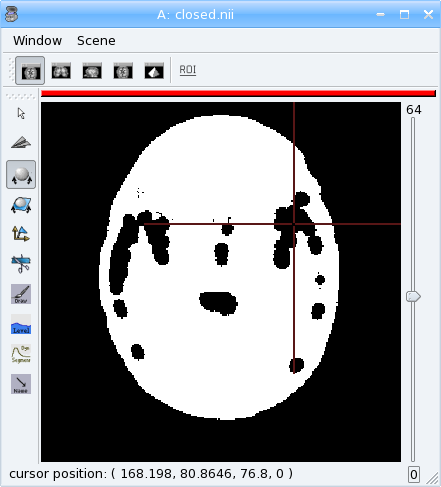
Mathematical morphology
[42]:
# apply 5mm closing
clvol = aimsalgo.AimsMorphoClosing(tvol, 5)
aims.write(clvol, 'closed.nii')
Mesher
[43]:
m = aimsalgo.Mesher()
mesh = aims.AimsSurfaceTriangle() # create an empty mesh
# the border should be -1
clvol.fillBorder(-1)
# get a smooth mesh of the interface of the biggest connected component
m.getBrain(clvol, mesh)
aims.write(mesh, 'head_mesh.gii')
reading slice      :   0  1  2  3  4  5  6  7  8  9 10 11 12 13 14 15 16 17 18 19 20 21 22 23 24 25 26 27 28 29 30 31 32 33 34 35 36 37 38 39 40 41 42 43 44 45 46 47 48 49 50 51 52 53 54 55 56 57 58 59 60 61 62 63 64 65 66 67 68 69 70 71 72 73 74 75 76 77 78 79 80 81 82 83 84 85 86 87 88 89 90 91 92 93 94 95 96 97 98 99100101102103104105106107108109110111112113114115116117118119120121122123124
getting interface  :     032767done
processing mesh    : reduced neighborhood  extended neighborhood vertices              smoothing  iteration     0    1    2    3    4    5    6    7    8    9   10   11   12   13   14   15   16   17   18   19   20   21   22   23   24   25   26   27   28   29   30                          pass 1/3 : decimating      0   100   200   300   400   500   600   700   800   900  1000  1100  1200  1300  1400  1500  1600  1700  1800  1900  2000  2100  2200  2300  2400  2500  2600  2700  2800  2900  3000  3100  3200  3300  3400  3500  3600  3700  3800  3900  4000  4100  4200  4300  4400  4500  4600  4700  4800  4900  5000  5100  5200  5300  5400  5500  5600  5700  5800  5900  6000  6100  6200  6300  6400  6500  6600  6700  6800  6900  7000  7100  7200  7300  7400  7500  7600  7700  7800  7900  8000  8100  8200  8300  8400  8500  8600  8700  8800  8900  9000  9100  9200  9300  9400  9500  9600  9700  9800  9900 10000 10100 10200 10300 10400 10500 10600 10700 10800 10900 11000 11100 11200 11300 11400 11500 11600 11700 11800 11900 12000 12100 12200 12300 12400 12500 12600 12700 12800 12900 13000 13100 13200 13300 13400 13500 13600 13700 13800 13900 14000 14100 14200 14300 14400 14500 14600 14700 14800 14900 15000 15100 15200 15300 15400 15500 15600 15700 15800 15900 16000 16100 16200 16300 16400 16500 16600 16700 16800 16900 17000 17100 17200 17300 17400 17500 17600 17700 17800 17900 18000 18100 18200 18300 18400 18500 18600 18700 18800 18900 19000 19100 19200 19300 19400 19500 19600 19700 19800 19900 20000 20100 20200 20300 20400 20500 20600 20700 20800 20900 21000 21100 21200 21300 21400 21500 21600 21700 21800 21900 22000 22100 22200 22300 22400 22500 22600 22700 22800 22900 23000 23100 23200 23300 23400 23500 23600 23700 23800 23900 24000 24100 24200 24300 24400 24500 24600 24700 24800 24900 25000 25100 25200 25300 25400 25500 25600 25700 25800 25900 26000 26100 26200 26300 26400 26500 26600 26700 26800 26900 27000 27100 27200 27300 27400 27500 27600 27700 27800 27900 28000 28100 28200 28300 28400 28500 pass 2/3 : decimating      0   100   200   300   400   500   600   700   800   900  1000  1100  1200  1300  1400  1500  1600  1700  1800  1900  2000  2100  2200  2300  2400  2500  2600  2700  2800  2900  3000  3100  3200  3300  3400  3500  3600  3700  3800  3900  4000  4100  4200  4300  4400  4500  4600  4700  4800  4900  5000  5100  5200  5300  5400  5500  5600  5700  5800  5900  6000  6100  6200  6300  6400  6500  6600  6700  6800  6900  7000  7100  7200  7300  7400  7500  7600  7700  7800  7900  8000  8100  8200  8300  8400  8500  8600  8700  8800  8900  9000  9100  9200  9300  9400  9500  9600  9700  9800  9900 10000 10100 10200 10300 10400 10500 10600 10700 10800 10900 11000 11100 11200 11300 11400 11500 11600 11700 11800 11900 12000 12100 12200 12300 12400 12500 12600 12700 12800 12900 13000 13100 13200 13300 13400 13500 13600 13700 13800 13900 14000 14100 14200 14300 14400 14500 14600 14700 14800 14900 15000 15100 15200 15300 15400 15500 15600 15700 15800 15900 16000 16100 16200 16300 16400 16500 16600 16700 16800 16900 17000 17100 17200 17300 17400 17500 17600 17700 17800 17900 18000 18100 18200 18300 18400 18500 18600 18700 18800 18900 19000 19100 19200 19300 19400 19500 19600 19700 19800 19900 20000 20100 20200 20300 20400 20500 20600 20700 20800 20900 21000 21100 21200 21300 21400 21500 21600 21700 21800 21900 22000 22100 22200 22300 22400 22500 22600 22700 22800 22900 23000 23100 23200 23300 23400 23500 23600 23700 23800 23900 24000 24100 24200 24300 24400 24500 24600 24700 24800 24900 25000 25100 25200 25300 25400 25500 25600 25700 25800 25900 26000 26100 26200 26300 26400 26500 26600 26700 26800 26900 27000 27100 27200 27300 27400 27500 27600 27700 27800 27900 28000 28100 28200 28300 28400 28500 28600 28700 28800 28900 29000 29100 29200 29300 29400 29500 29600 29700 29800 29900 30000 30100 30200 30300 30400 30500 30600 30700 30800 30900 31000 31100 31200 31300 31400 31500 31600 31700 31800 31900 32000 32100 32200 32300 32400 32500 32600 32700 32800 32900 33000 33100 33200 33300 33400 33500 33600 33700 33800 33900 34000 34100 34200 34300 34400 34500 34600 34700 34800 34900 35000 35100 35200 35300 35400 35500 35600 35700 35800 35900 36000 36100 36200 36300 36400 36500 36600 36700 36800 36900 37000 37100 37200 37300 37400 37500 37600 37700 37800 37900 38000 38100 38200 38300 38400 38500 38600 38700 38800 38900 39000 39100 39200 39300 39400 39500 39600 39700 39800 39900 40000 40100 40200 40300 40400 40500 40600 40700 40800 40900 41000 41100 41200 41300 41400 41500 41600 41700 41800 41900 42000 42100 42200 42300 42400 42500 42600 42700 42800 42900 43000 43100 43200 43300 43400 43500 43600 43700 43800 43900 44000 44100 44200 44300 44400 44500 44600 44700 44800 44900 45000 45100 45200 45300 45400 45500 45600 45700 45800 45900 46000 46100 46200 46300 46400 46500 46600 46700 46800 46900 47000 47100 47200 47300 47400 47500 47600 47700 47800 47900 48000 48100 48200 48300 48400 48500 48600 48700 48800 48900 49000 49100 49200 49300 49400 49500 49600 49700 49800 49900 50000 50100 50200 50300 50400 50500 50600 50700 50800 50900 51000 51100 51200 51300 51400 51500 51600 51700 51800 51900 52000 52100 52200 52300 52400 52500 52600 52700 52800 52900 53000 53100 53200 53300 53400 53500 53600 53700 53800 53900 54000 54100 54200 54300 54400 54500 54600 54700 54800 54900 55000 55100 55200 55300 55400 55500 55600 55700 55800 55900 56000 56100 56200 56300 56400 56500 56600 56700 56800 56900 57000 57100 57200 57300 57400 57500 57600 57700 57800 57900 58000 58100 58200 58300 58400 58500 58600 58700 58800 58900 59000 59100 59200 59300 59400 59500 59600 59700 59800 59900 60000 60100 60200 60300 60400 60500 60600 60700 60800 60900 61000 61100 61200 61300 61400 61500 61600 61700 61800 61900 62000 62100 62200 62300 62400 62500 62600 62700 62800 62900 63000 63100 63200 63300 63400 63500 63600 63700 63800 63900 64000 64100 64200 64300 64400 64500 64600 64700 64800 64900 65000 65100 65200 65300 65400 65500 65600 65700 65800 65900 66000 66100 66200 66300 66400 66500 66600 66700 66800 66900 67000 67100 67200 67300 67400 67500 67600 67700 67800 67900 68000 68100 68200 68300 68400 68500 68600 68700 68800 68900 69000 69100 69200 69300 69400 69500 69600 69700 69800 69900 70000 70100 70200 70300 70400 70500 70600 70700 70800 70900 71000 71100 71200 71300 71400 71500 71600 71700 71800 71900 72000 72100 72200 72300 72400 72500 72600 72700 72800 72900 73000 73100 pass 3/3 : decimating      0   100   200   300   400   500   600   700   800   900  1000  1100  1200  1300  1400  1500  1600  1700  1800  1900  2000  2100  2200  2300  2400  2500  2600  2700  2800  2900  3000  3100  3200  3300  3400  3500  3600  3700  3800  3900  4000  4100  4200  4300  4400  4500  4600  4700  4800  4900  5000  5100  5200  5300  5400  5500  5600  5700  5800  5900  6000  6100  6200  6300  6400  6500  6600  6700  6800  6900  7000  7100  7200  7300  7400  7500  7600  7700  7800  7900  8000  8100  8200  8300  8400  8500  8600  8700  8800  8900  9000  9100  9200  9300  9400  9500  9600  9700  9800  9900 10000 10100 10200 10300 10400 10500 10600 10700 10800 10900 11000 11100 11200 11300 11400 11500 11600 11700 11800 11900 12000 12100 12200 12300 12400 12500 12600 12700 12800 12900 13000 13100 13200 13300 13400 13500 13600 13700 13800 13900 14000 14100 14200 14300 14400 14500 14600 14700 14800 14900 15000 15100 15200 15300 15400 15500 15600 15700 15800 15900 16000 16100 16200 16300 16400 16500 16600 16700 16800 16900 17000 17100 17200 17300 17400 17500 17600 17700 17800 17900 18000 18100 18200 18300 18400 18500 18600 18700 18800 18900 19000 19100 19200 19300 19400 19500 19600 19700 19800 19900 20000 20100 20200 20300 20400 20500 20600 20700 20800 20900 21000 21100 21200 21300 21400 21500 21600 21700 21800 21900 22000 22100 22200 22300 22400 22500 22600 22700 22800 22900 23000 23100 23200 23300 23400 23500 23600 23700 23800 23900 24000 24100 24200 24300 24400 24500 24600 24700 24800 24900 25000 25100 25200 25300 25400 25500 25600 25700 25800 25900 26000 26100 26200 26300 26400 26500 26600 26700 26800 26900 27000 27100 27200 27300 27400 27500 27600 27700 27800 27900 28000 28100 28200 28300 28400 28500 28600 28700 28800 28900 29000 29100 29200 29300 29400 29500 29600 29700 29800 29900 30000 30100 30200 30300 30400 30500 30600 30700 30800 30900 31000 31100 31200 31300 31400 31500 31600 31700 31800 31900 32000 32100 32200 32300 32400 32500 32600 32700 32800 32900 33000 33100 33200 33300 33400 33500 33600 33700 33800 33900 34000 34100 34200 34300 34400 34500 34600 34700 34800 34900 35000 35100 35200 35300 35400 35500 35600 35700 35800 35900 36000 36100 36200 36300 36400 36500 36600 36700 36800 36900 37000 37100 37200 37300 37400 37500 37600 37700 37800 37900 38000 38100 38200 38300 38400 38500 38600 38700 38800 38900 39000 39100 39200 39300 39400 39500 39600 39700 39800 39900 40000 40100 40200 40300 40400 40500 40600 40700 40800 40900 41000 41100 41200 41300 41400 41500 41600 41700 41800 41900 42000 42100 42200 42300 42400 42500 42600 42700 42800 42900 43000 43100 43200 43300 43400 43500 43600 43700 43800 43900 44000 44100 44200 44300 44400 44500 44600 44700 44800 44900 45000 45100 45200 45300 45400 45500 45600 45700 45800 45900 46000 46100 46200 46300 46400 46500 46600 46700 46800 46900 47000 47100 47200 47300 47400 47500 47600 47700 47800 47900 48000 48100 48200 48300 48400 48500 48600 48700 48800 48900 49000 49100 49200 49300 49400 49500 49600 49700 49800 49900 50000 50100 50200 50300 50400 50500 50600 50700 50800 50900 51000 51100 51200 51300 51400 51500 51600 51700 51800 51900 52000 52100 52200 52300 52400 52500 52600 52700 52800 52900 53000 53100 53200 53300 53400 53500 53600 53700 53800 53900 54000 54100 54200 54300 54400 54500 54600 54700 54800 54900 55000 55100 55200 55300 55400 55500 55600 55700 55800 55900 56000 56100 56200 56300 56400 56500 56600 56700 56800 56900 57000 57100 57200 57300 57400 57500 57600 57700 57800 57900 58000 58100 58200 58300 58400 58500 58600 58700 58800 58900 59000 59100 59200 59300 59400 59500 59600 59700 59800 59900 60000 60100 60200 60300 60400 60500 60600 60700 60800 60900 61000 61100 61200 61300 61400 61500 61600 61700 61800 61900 62000 62100 62200 62300 62400 62500 62600 62700 62800 62900 63000 63100 63200 63300 63400 63500 63600 63700 63800 63900 64000 64100 64200 64300 64400 64500 64600 64700 64800 64900 65000 65100 65200 65300 65400 65500 65600 65700 65800 65900 66000 66100 66200 66300 66400 66500 66600 66700 66800 66900 67000 67100 67200 67300 67400 67500 67600 67700 67800 67900 68000 68100 68200 68300 68400 68500 68600 68700 68800 68900 69000 69100 69200 69300 69400 69500 69600 69700 69800 69900 70000 70100 70200 70300 70400 70500 70600 70700 70800 70900 71000 71100 71200 71300 71400 71500 71600 71700 71800 71900 72000 72100 72200 72300 72400 72500 72600 72700 72800 72900 73000 73100 73200 73300 73400 73500 73600 73700 73800 73900 74000 74100 74200 74300 74400 74500 74600 74700 74800 74900 75000 75100 75200 75300 75400 75500 75600 75700 75800 75900 76000 76100 76200 76300 76400 76500 76600 76700 76800 76900 77000 77100 77200 77300 77400 77500 77600 77700 77800 77900 78000 78100 78200 78300 78400 78500 78600 78700 78800 78900 79000 79100 79200 79300 79400 79500 79600 79700 79800 79900 80000 80100 80200 80300 80400 80500 80600 80700 80800 80900 81000 81100 81200 81300 81400 81500 81600 81700 81800 81900 82000 82100 82200 82300 82400 82500 82600 82700 82800 82900 83000 83100 83200 83300 83400 83500 83600 83700 83800 83900 84000 84100 84200 84300 84400 84500 84600 84700 84800 84900 85000 85100 85200 85300 85400 85500 85600 85700 85800 85900 86000 86100 86200 86300 86400 86500 86600 86700 smoothing  iteration     0    1    2    3    4    5    6    7    8    9   10   11   12   13   14   15   16   17   18   19   20   21   22   23   24   25   26   27   28   29   30                          normals               triangles             done ( 62.5473% reduction )
clearing interface : done
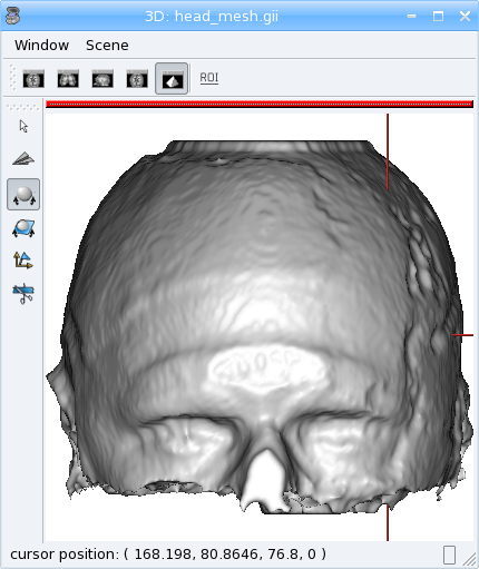
The above examples make up a simplified version of the head mesh extraction algorithm in VipGetHead, used in the Morphologist pipeline.
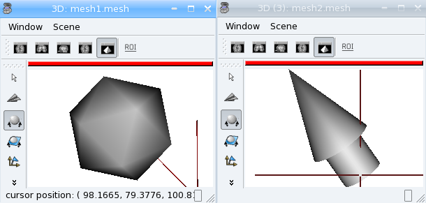
Surface generation
The soma.aims.SurfaceGenerator allows to create simple meshes of predefined shapes: cube, cylinder, sphere, icosehedron, cone, arrow.
[44]:
from soma import aims
center = (50, 25, 20)
radius = 53
mesh1 = aims.SurfaceGenerator.icosahedron(center, radius)
mesh2 = aims.SurfaceGenerator.generate(
    {'type': 'arrow', 'point1': [30, 70, 0],
     'point2': [100, 100, 100], 'radius': 20, 'arrow_radius': 30,
     'arrow_length_factor': 0.7, 'facets': 50})
# get the list of all possible generated objects and parameters:
print(aims.SurfaceGenerator.description())
assert('arrow_length_factor' in aims.SurfaceGenerator.description()[0])
[ { 'arrow_length_factor' : 'relative length of the head', 'arrow_radius' : 'radius of the tail', 'facets' : '(optional) number of facets of the cone section (default: 4)', 'point1' : '3D position of the head', 'point2' : '3D position of the center of the bottom', 'radius' : 'radius of the head', 'type' : 'arrow' }, { 'closed' : '(optional) if non-zero, make polygons for the cone end (default: 0)', 'facets' : '(optional) number of facets of the cone section (default: 4)', 'point1' : '3D position of the sharp end', 'point2' : '3D position of the center of the other end', 'radius' : 'radius of the 2nd end', 'smooth' : '(optional) make smooth normals and shared vertices (default: 0)', 'type' : 'cone' }, { 'center' : '3D position of the center', 'radius' : 'half-length of the edge', 'smooth' : '(optional) make smooth normals and shared vertices (default: 0)', 'type' : 'cube' }, { 'closed' : '(optional) if non-zero, make polygons for the cylinder ends (default: 0)', 'facets' : '(optional) number of facets of the cylinder section (default: 4)', 'point1' : '3D position of the center of the 1st end', 'point2' : '3D position of the center of the 2nd end', 'radius' : 'radius of the 1st end', 'radius2' : '(optional) radius of the 2nd end (default: same as radius)', 'smooth' : '(optional) make smooth normals and shared vertices for the tube part (default: 1)', 'type' : 'cylinder' }, { 'center' : '3D position of the center, may also be specified as \'point1\' parameter', 'facets' : '(optional) number of facets of the sphere. May also be specified as \'nfacets\' parameter (default: 225)', 'radius1' : 'radius1', 'radius2' : 'radius2', 'type' : 'ellipse', 'uniquevertices' : '(optional) if set to 1, the pole vertices are not duplicated( default: 0)' }, { 'center' : '3D position of the center', 'radius' : 'radius', 'type' : 'icosahedron' }, { 'center' : '3D position of the center, may also be specified as \'point1\' parameter', 'facets' : '(optional) minimum number of facets of the sphere. (default: 30)', 'radius' : 'radius', 'type' : 'icosphere' }, { 'boundingbox_max' : '3D position of the higher bounding box', 'boundingbox_min' : '3D position of the lower bounding box', 'smooth' : '(optional) make smooth normals and shared vertices (default: 0)', 'type' : 'parallelepiped' }, { 'center' : '3D position of the center, may also be specified as \'point1\' parameter', 'facets' : '(optional) number of facets of the sphere. May also be specified as \'nfacets\' parameter (default: 225)', 'radius' : 'radius', 'type' : 'sphere', 'uniquevertices' : '(optional) if set to 1, the pole vertices are not duplicated( default: 0)' } ]
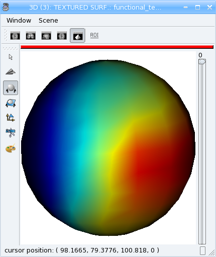
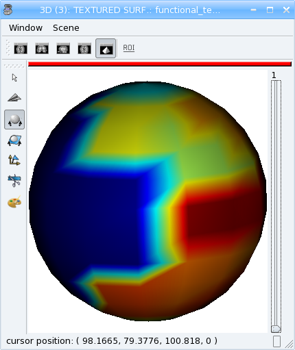
Interpolation
Interpolators help to get values in millimeters coordinates in a discrete space (volume grid), and may allow voxels values mixing (linear interpolation, typically).
[45]:
from soma import aims
import numpy as np
# load a functional volume
vol = aims.read('data_for_anatomist/subject01/Audio-Video_T_map.nii')
# get the position of the maximum
maxval = vol.max()
pmax = [p[0] for p in np.where(vol.np == maxval)]
# set pmax in mm
vs = vol.header()['voxel_size']
pmax = [x * y for x,y in zip(pmax, vs)]
# take a sphere of 5mm radius, with about 200 vertices
mesh = aims.SurfaceGenerator.sphere(pmax[:3], 5., 200)
vert = mesh.vertex()
# get an interpolator
interpolator = aims.aims.getLinearInterpolator(vol)
# create a texture for that sphere
tex = aims.TimeTexture_FLOAT()
tx = tex[0]
tx2 = tex[1]
tx.reserve(len(vert))
tx2.reserve(len(vert))
for v in vert:
    tx.append(interpolator.value(v))
    # compare to non-interpolated value
    tx2.append(vol.value(*[int(round(x / y)) for x,y in zip(v, vs)]))
aims.write(tex, 'functional_tex.gii')
aims.write(mesh, 'sphere.gii')
Look at the difference between the two timesteps (interpolated and non-interpolated) of the texture in Anatomist.
Types conversion
The Converter_*_* classes allow to convert some data structures types to others. Of course all types cannot be converted to any other, but they are typically used ton convert volumed from a given voxel type to another one. A “factory” function may help to build the correct converter using input and output types. For instance, to convert the anatomical volume of the previous examples to float type:
[46]:
from soma import aims
vol = aims.read('data_for_anatomist/subject01/subject01.nii')
print('type of vol:', type(vol))
assert(type(vol) is aims.Volume_S16)
c = aims.Converter(intype=vol, outtype=aims.Volume('FLOAT'))
vol2 = c(vol)
print('type of converted volume:', type(vol2))
assert(type(vol2) is aims.Volume_FLOAT)
print('value of initial volume at voxel (50, 50, 50):', vol.value(50, 50, 50))
assert(vol.value(50, 50, 50) == 57)
print('value of converted volume at voxel (50, 50, 50):', vol2.value(50, 50, 50))
assert(vol2.value(50, 50, 50) == 57.0)
type of vol: <class 'soma.aims.Volume_S16'>
type of converted volume: <class 'soma.aims.Volume_FLOAT'>
value of initial volume at voxel (50, 50, 50): 57
value of converted volume at voxel (50, 50, 50): 57.0
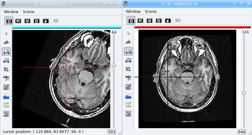
Resampling
Resampling allows to apply a geometric transformation or/and to change voxels size. Several types of resampling may be used depending on how we interpolate values between neighbouring voxels (see interpolators): nearest-neighbour (order 0), linear (order 1), spline resampling with order 2 to 7 in AIMS.
[47]:
from soma import aims, aimsalgo
import math
vol = aims.read('data_for_anatomist/subject01/subject01.nii')
# create an affine transformation matrix
# rotating pi/8 along z axis
tr = aims.AffineTransformation3d(aims.Quaternion([0, 0, math.sin(math.pi / 16), math.cos(math.pi / 16)]))
tr.setTranslation((100, -50, 0))
# get an order 2 resampler for volumes of S16
resp = aims.ResamplerFactory_S16().getResampler(2)
resp.setDefaultValue(-1) # set background to -1
resp.setRef(vol) # volume to resample
# resample into a volume of dimension 200x200x200 with voxel size 1.1, 1.1, 1.5
resampled = resp.doit(tr, 200, 200, 200, (1.1, 1.1, 1.5))
# Note that the header transformations to external referentials have been updated
print(resampled.header()['referentials'])
assert(resampled.header()['referentials']
       == ['Scanner-based anatomical coordinates', 'Talairach-MNI template-SPM'])
import numpy
numpy.set_printoptions(precision=4)
for t in resampled.header()['transformations']:
    print(aims.AffineTransformation3d(t))
aims.write(resampled, 'resampled.nii')
  0 %  1 %  2 %  3 %  4 %  5 %  6 %  7 %  8 %  9 % 10 % 11 % 12 % 13 % 14 % 15 % 16 % 17 % 18 % 19 % 20 % 21 % 22 % 23 % 24 % 25 % 26 % 27 % 28 % 29 % 30 % 31 % 32 % 33 % 34 % 35 % 36 % 37 % 38 % 39 % 40 % 41 % 42 % 43 % 44 % 45 % 46 % 47 % 48 % 49 % 50 % 51 % 52 % 53 % 54 % 55 % 56 % 57 % 58 % 59 % 60 % 61 % 62 % 63 % 64 % 65 % 66 % 67 % 68 % 69 % 70 % 71 % 72 % 73 % 74 % 75 % 76 % 77 % 78 % 79 % 80 % 81 % 82 % 83 % 84 % 85 % 86 % 87 % 88 % 89 % 90 % 91 % 92 % 93 % 94 % 95 % 96 % 97 % 98 % 99 %100 %["Scanner-based anatomical coordinates", "Talairach-MNI template-SPM"]
[[ -0.9239  -0.3827   0.     193.2538]
 [  0.3827  -0.9239   0.      34.6002]
 [  0.       0.      -1.      73.1996]
 [  0.       0.       0.       1.    ]]
[[-9.6797e-01 -4.1623e-01  1.0548e-02  2.0329e+02]
 [ 3.8418e-01 -8.9829e-01  3.6210e-02  2.8707e+00]
 [ 3.9643e-03 -2.0773e-02 -1.2116e+00  9.3405e+01]
 [ 0.0000e+00  0.0000e+00  0.0000e+00  1.0000e+00]]
Load the original image and the resampled in Anatomist. See how the resampled has been rotated. Now apply the NIFTI/SPM referential info on both images. They are now aligned again, and cursor clicks correctly go to the same location on both volume, whatever the display referential for each of them.
PyAIMS / PyAnatomist integration
It is possible to use both PyAims and PyAnatomist APIs together in python. See the Pyanatomist / PyAims tutorial.
At the end, cleanup the temporary working directory
[48]:
# cleanup data
import shutil
os.chdir(older_cwd)
shutil.rmtree(tuto_dir)