Cortical Fold Arg (3.0)

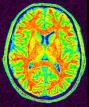
Compute the graph of the cortical folds

Description

This procedure compresses the T1-weighted MR image into a structure, which sums up the main information about the cortical folding patterns. The goal is a filtering of the huge amount of information embedded into the grey levels in order to build a simplified representation sufficient to perform the recognition of cortical sulci or sulcal roots. This representation is a graph, which nodes correspond to elementary cortical folds, and which links correspond to the relative topographies of these folds. This representation allows us to deal with folding patterns in an abstract way more adapted to pattern recognition technics that try to mimic the neuroanatomist's approach: the entities of interest are no more the voxels and their grey levels but the cortical folds, their sizes and orientations, possible connexions, etc...

For instance, here is the graph based representation of a relatively simple sulcus:

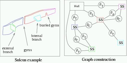
The sulcus is split into 5 elementary folds, which are represented by the graph nodes (the squares). The external hull of the brain is also represented by a graph node. Finally, the relations between these nodes (the circles) represent various topographical information:

1. T represents a junction between two folds or one fold and the brain hull;
2. C represents a neighborhood relationship geodesical to the brain hull : a direct path exists on the cortical surface between the two folds. This neighborhood corresponds to adjacencies in a Voronoï diagram geodesic to the brain hull and computed for the junctions with this hull. This diagram is a parcelling of the hull relative to the nearest junction. Each elementary fold is endowed with an influence zone around it. Two folds are linked if their relative zones touch each other;
3. P represents the anatomical "pli de passage" notion described during the XIXth century. This notion corresponds to some gyri that are usually burried into the depth of a sulcus, but may reach the brain hull in some individuals and hence split the sulcus. These burried gyri are detected from depth and cortical surface curvature criteria.

The graph construction relies on a long processing line:

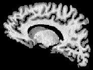
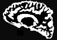
1. The grey/white interface is detected first as a spherical surface. The underlying algorithm uses a mask of each hemisphere yielded by Ana Split Brain From Brain Mask:
   
   This mask is embedded into a parallelepipedic box, which inner interface deforms itself in order to reach the grey/white interface, and which outer interface reaches the hemisphere hull:
   
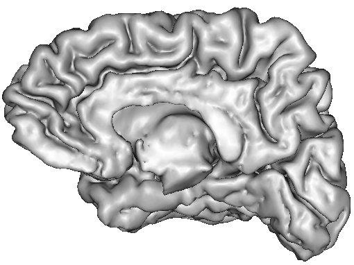
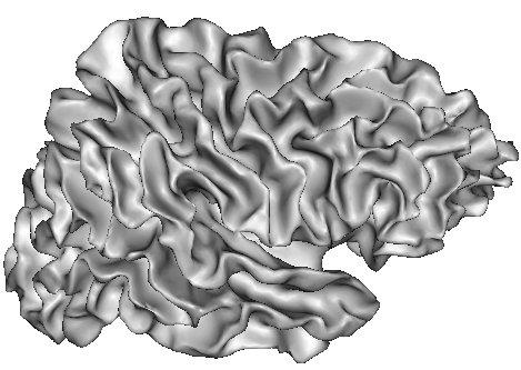
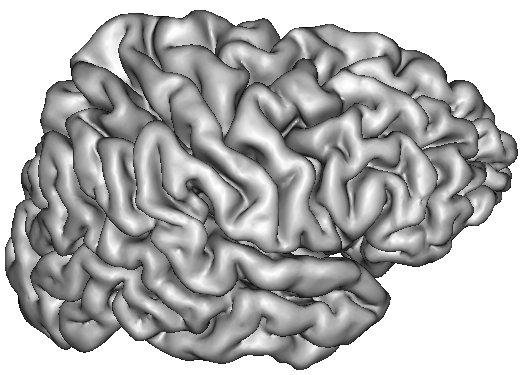
   The resulting grey/white interface can be converted into a mesh endowed with the spherical topology, which will be inflated by some other Brainvisa treatments for visualization purpose (Ana Inflate Cortical Surface):
   
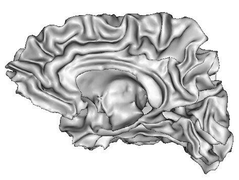
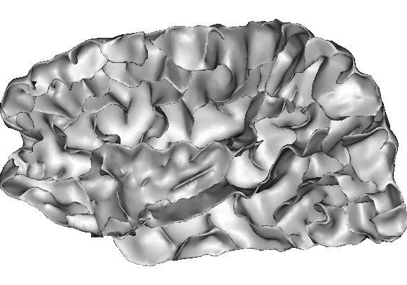
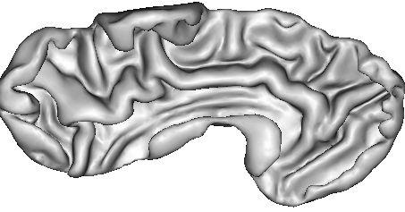
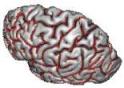
   A dilation of this interface towards the outer brain edges may lead to nice 3D rendering of the cortical surface, which are easy to read because the folds are opened (Ana Get Opened Hemi Surface) :
   
   
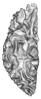
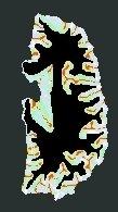
2. The next stage consists of a skeletonization of the white object mentioned above. This object is eroded from the inside until no more "flesh" remains. The final skeleton looks like a negative mold of the brain, or like the husk of a Grenoble nut.
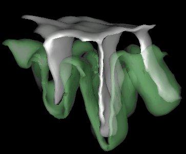
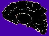
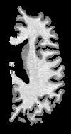
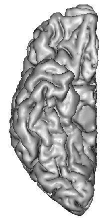
   Imagine that a cerebral hemisphere has been split in two, and that white matter has been removed. The cortical surface can then be visualised from the inside:
   
   
   This point of view helps to understand he skeletonization effect:
   
   
   The skeleton is made up of the the brain hull and of the numerous surfaces medial to the folds:
   
   
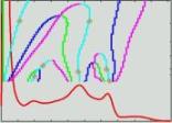
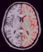
   In fact, the erosion applied to compute the skeleton has not a uniform speed. To deal with variable cortex thicknesses on both sides of the fold, and to master the final depth of the skeleton, the grey levels of the MR image are used to define the localization of the skeleton. Let us imagine that the grey level is an altitude, white matter is the mountain's crests, cerebro spinal fluid is the mountain's crevasses. To impose the skeleton localization in the depth of the crevasses, we use a "crevasse detector", the mean curvature of the MR image isosurfaces:
   
   
   This detector is not perfect: some of the crevasse's points are lost. The algorithm used to perform the skeletonization, however, can fill the holes in the crevasse surfaces (technically, it is a homotopic erosion). This erosion's effect looks like the effect of tide on sand castles. The castle's altitude at each point corresponds to the crevasse detector answer. Each wave will remove some sand of the castle's outside walls. Little by little, the walls will collapse under the water level. The highest parts of the castle will be the last to collapse. When two water fronts meet at the same place, a skeleton point is created:
   
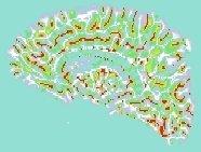
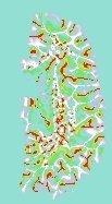
   The crevasse detector:
   
   
   The final skeleton (colors correspond to a topological classification of the fold junctions and of the fold bottoms):
   
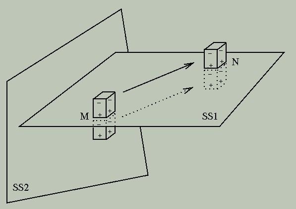
   The visualization of 2D slices is rather disturbing, because it is difficult to understand that the skeleton has kept the spherical topology (more precisely, the homotopy of a sphere...)
3. Next step (if you are not fed up yet...): the goal of the skeletonization is to reach a point, where the elementary fold extraction is simple. The skeleton can be split at the level of junctions to get the puzzle toy we need. This operation is performed using a discrete topology technic, which may be understood from the following metaphor. Let us imagine two magnets stick together on both sides of a skeleton's surface:
   
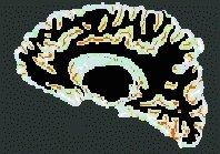
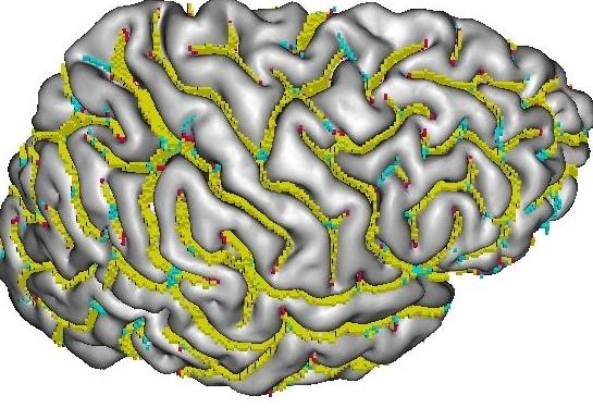
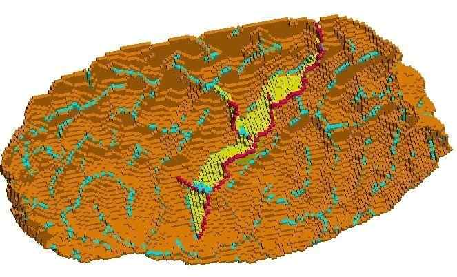
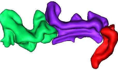
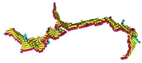
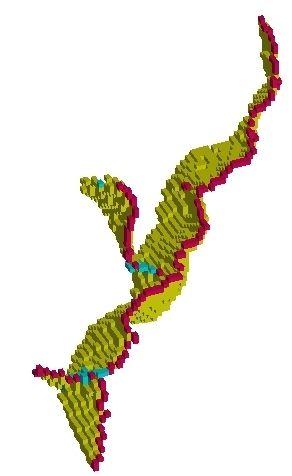
   All the surface points, which can be reached when the two magnets slide together, are gathered into the same elementary fold. Using the discrete topology's jargon, these skeleton subsets are called simple surfaces. This parcelling is applied to the subset of skeleton points, which split the background into two connected components. This subset discards fold bottoms and most of the junction points (unfortunately, no exhaustive junction detector has been proposed up to now, as far as we are aware...). This surface points are yellow:
   
   
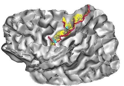
   Zoom on a skeleton piece:
   
   
   Only the brain hull survives in orange :
   
   
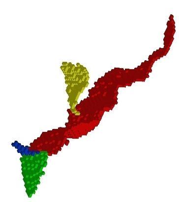
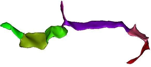
   The parcelling:
   
   
   
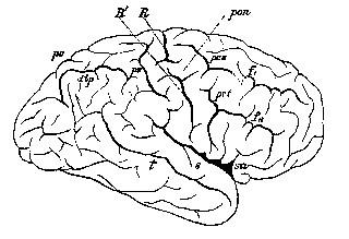
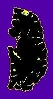
4. Last step, the detection of the putative burried gyri. The goal is to add into the cortex folding representation the necessary information to study the sulcal root notion. We are aiming indeed at defining a model of the cortical folding patterns built upon indivisible elementary units that may correspond to the first folds appearing during in utero life. This research program wants to overcome the weaknesses of the usual descriptions of the sulcus interruptions, a phenomenon which can even occur for the central sulcus:
   
   
   We try to split the central sulcus at the level of the middle "pli de passage", which defines the two underlying sulcal roots. Viewed from beneath:
   
   
   The simple surfaces are split into several pieces when depth variations or high values of the Gaussian curvature are clues of some putative gyrus. The current procedure is still far to be fully satisfying. Current efforts to improve it may be found in:
   
   A mean curvature based primal sketch to study the cortical folding process from antenatal to adult brain.
   A. Cachia, J.-F. Mangin, D. Rivière, N. Boddaert, A. Andrade, F. Kherif, P. Sonigo, D. Papadopoulos-Orfanos, M. Zilbovicius, J.-B. Poline, I. Bloch, F. Brunelle, and J. Régis.
   In MICCAI, Utrecht, The Netherlands, LNCS-2208, pages 897--904. Springer Verlag, 2001.
   
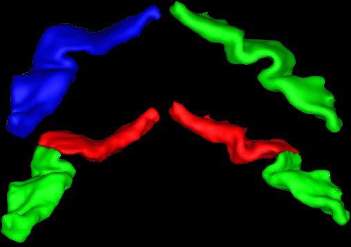
   Here are a few images to help to understand the splitting process at the level of Calloso marginal fissure:
   
   
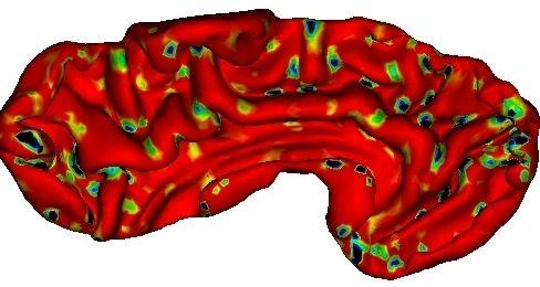
   Geodesic depth :
   
   
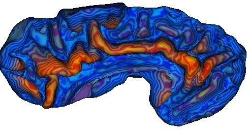
   Gaussian curvature of the cortical surface, which gives information about saddle points that may be related to burried gyri:
   
   
   The parceling stemming from the burried gyri:
   
   
   The skeleton :
   
   
   The final segmentation, which mixes the simple surface and burried gyrus notions
   
   
   Yes I know, it is a lot of pieces...

For the neurotic reader, who really wants to know more:

From 3D magnetic resonance images to structural representations of the cortex topography using topology preserving deformations.
J.-F. Mangin, V. Frouin, I. Bloch, J. Regis, and J.Lopez-Krahe.
Journal of Mathematical Imaging and Vision, 5(4):297--318,1995.

Automatic recognition of cortical sulci of the human brain using a congregation of neural networks.
D. Rivière, J.-F. Mangin, D. Papadopoulos-Orfanos, J.-M. Martinez, V. Frouin, and J. Régis.
Medical Image Analysis, 6(2), pp 77-92 I

Parameters

Side: Choice ( input )

One or two hemispheres

mri_corrected: T1 MRI Bias Corrected ( input )

histo_analysis: Histo Analysis ( input )

split_mask: Split Brain Mask ( input )

left_hemi_cortex: Left CSF+GREY Mask ( output )

right_hemi_cortex: Right CSF+GREY Mask ( output )

detection of grey/white interface

Lskeleton: Left Cortex Skeleton ( output )

Skeleton of the previous object

Rskeleton: Right Cortex Skeleton ( output )

Lroots: Left Cortex Catchment Bassins ( output )

Bassins of a watershed

Rroots: Right Cortex Catchment Bassins ( output )

Lgraph: Cortical folds graph ( output )

Rgraph: Cortical folds graph ( output )

Commissure_coordinates: Commissure coordinates ( input )

compute_fold_meshes: Choice ( input )

Technical information

Toolbox : Morphologist

User level : 2

Identifier : AnaComputeCorticalFoldArg

File name : brainvisa/toolboxes/morphologist/processes/segmentationpipeline/components_obsolete/segmentation/AnaComputeCorticalFoldArg.py

Supported file formats :

mri_corrected :

gz compressed NIFTI-1 image, Aperio svs, BMP image, DICOM image, Directory, ECAT i image, ECAT v image, FDF image, FreesurferMGH, FreesurferMGZ, GIF image, GIS image, Hamamatsu ndpi, Hamamatsu vms, Hamamatsu vmu, JPEG image, Leica scn, MINC image, NIFTI-1 image, PBM image, PGM image, PNG image, PPM image, SPM image, Sakura svslide, TIFF image, TIFF image, TIFF(.tif) image, TIFF(.tif) image, VIDA image, Ventana bif, XBM image, XPM image, Zeiss czi, gz compressed MINC image, gz compressed NIFTI-1 image

histo_analysis :

Histo Analysis, Histo Analysis

split_mask :

gz compressed NIFTI-1 image, Aperio svs, BMP image, DICOM image, Directory, ECAT i image, ECAT v image, FDF image, FreesurferMGH, FreesurferMGZ, GIF image, GIS image, Hamamatsu ndpi, Hamamatsu vms, Hamamatsu vmu, JPEG image, Leica scn, MINC image, NIFTI-1 image, PBM image, PGM image, PNG image, PPM image, SPM image, Sakura svslide, TIFF image, TIFF image, TIFF(.tif) image, TIFF(.tif) image, VIDA image, Ventana bif, XBM image, XPM image, Zeiss czi, gz compressed MINC image, gz compressed NIFTI-1 image

left_hemi_cortex :

gz compressed NIFTI-1 image, BMP image, DICOM image, Directory, ECAT i image, ECAT v image, FDF image, GIF image, GIS image, JPEG image, MINC image, NIFTI-1 image, PBM image, PGM image, PNG image, PPM image, SPM image, TIFF image, TIFF(.tif) image, VIDA image, XBM image, XPM image, gz compressed MINC image, gz compressed NIFTI-1 image

right_hemi_cortex :

gz compressed NIFTI-1 image, BMP image, DICOM image, Directory, ECAT i image, ECAT v image, FDF image, GIF image, GIS image, JPEG image, MINC image, NIFTI-1 image, PBM image, PGM image, PNG image, PPM image, SPM image, TIFF image, TIFF(.tif) image, VIDA image, XBM image, XPM image, gz compressed MINC image, gz compressed NIFTI-1 image

Lskeleton :

gz compressed NIFTI-1 image, BMP image, DICOM image, Directory, ECAT i image, ECAT v image, FDF image, GIF image, GIS image, JPEG image, MINC image, NIFTI-1 image, PBM image, PGM image, PNG image, PPM image, SPM image, TIFF image, TIFF(.tif) image, VIDA image, XBM image, XPM image, gz compressed MINC image, gz compressed NIFTI-1 image

Rskeleton :

gz compressed NIFTI-1 image, BMP image, DICOM image, Directory, ECAT i image, ECAT v image, FDF image, GIF image, GIS image, JPEG image, MINC image, NIFTI-1 image, PBM image, PGM image, PNG image, PPM image, SPM image, TIFF image, TIFF(.tif) image, VIDA image, XBM image, XPM image, gz compressed MINC image, gz compressed NIFTI-1 image

Lroots :

gz compressed NIFTI-1 image, BMP image, DICOM image, Directory, ECAT i image, ECAT v image, FDF image, GIF image, GIS image, JPEG image, MINC image, NIFTI-1 image, PBM image, PGM image, PNG image, PPM image, SPM image, TIFF image, TIFF(.tif) image, VIDA image, XBM image, XPM image, gz compressed MINC image, gz compressed NIFTI-1 image

Rroots :

gz compressed NIFTI-1 image, BMP image, DICOM image, Directory, ECAT i image, ECAT v image, FDF image, GIF image, GIS image, JPEG image, MINC image, NIFTI-1 image, PBM image, PGM image, PNG image, PPM image, SPM image, TIFF image, TIFF(.tif) image, VIDA image, XBM image, XPM image, gz compressed MINC image, gz compressed NIFTI-1 image

Lgraph :

Graph and data, Graph and data

Rgraph :

Graph and data, Graph and data

Commissure_coordinates :

Commissure coordinates, Commissure coordinates